Determination of optical properties by interstitial white light spectroscopy using a custom fiber optic probe

Timothy M. Baran; Michael C. Fenn; Thomas H. Foster

doi:10.1117/1.JBO.18.10.107007

22 October 2013 Determination of optical properties by interstitial white light spectroscopy using a custom fiber optic probe

Timothy M. Baran, Michael C. Fenn, Thomas H. Foster

Author Affiliations +

Journal of Biomedical Optics, Vol. 18, Issue 10, 107007 (October 2013). https://doi.org/10.1117/1.JBO.18.10.107007

Abstract

We demonstrate interstitial recovery of absorption and scattering coefficients using a custom optical probe and a Monte Carlo (MC)–based recovery algorithm. The probe consists of six side-firing spectroscopy fibers contained in a 1.1-mm outer diameter cladding, with each fiber having a different axial and angular position on the probe. Broadband white light is delivered by one of the fibers and is detected steady-state by the remaining fibers. These spatially and spectrally resolved data are analyzed using a MC-based fitting algorithm in order to extract the local optical properties. The technique was verified in tissue-simulating phantoms consisting of Intralipid-20% as a scatterer and either manganese meso-tetra (4-sulfanatophenyl) porphine or intact human erythrocytes as an absorber. Absorption coefficients were recovered with a mean error of 9% and scattering coefficients were recovered with a mean error of 19%, whereas the hemoglobin oxygen saturation was recovered with a mean error of 12%. These results demonstrate the feasibility of optical property recovery for situations in which surface-contact spectroscopy is not a possibility, and where only a single probe can be inserted into the tissue.

1. Introduction

Steady-state reflectance spectroscopy using surface-contact or off-surface measurements has been used extensively to determine the absorption ( $μ_{a}$ ) and reduced scattering ( $μ_{s}^{'}$ ) coefficients of biological tissue. In this scenario, broadband light is injected into the tissue at a given point on the surface and detected at one or more positions. A model of light propagation is then utilized to extract the optical properties of the sample based on the light detected. There has been a large volume of work done on this topic, with numerous studies detailing recovery of optical properties from spatially resolved measurements.¹^–³ Our laboratory has also done significant work on the recovery of optical properties from surface measurements of diffuse reflectance.⁴^–⁶

These techniques are limited in their applicability, however, due to the requirement that the tissue in question be accessible to surface measurements. Due to the absorptive and highly scattering nature of tissue, light propagation is limited to regions that are close to the source and detectors. An excellent analysis of the regions sampled by steady-state diffuse reflectance for a particular source–detector configuration is provided by Feng et al.⁷ In the weak absorption limit, they give $z = d \sqrt{2} / 4$ as the maximum depth of sensitivity, where $d$ is the source–detector separation. For a typical source–detector separation of 10 mm, this yields a maximum depth sensitivity of $\sim 3.5 mm$ in this limit. In the strong absorption limit, this maximum depth changes to $z = \sqrt{d / 2 μ_{eff}}$ , where $μ_{eff}$ is the effective attenuation coefficient defined as $μ_{eff} = \sqrt{3 μ_{a} (μ_{a} + μ_{s}^{'})}$ .

For certain applications, it is desirable to know the optical properties of a tissue volume that cannot be sampled by surface spectroscopy. There has been a good deal of work done on this topic, with solutions being roughly separated into two categories. The first of these uses an array of individual spectroscopy fibers that are inserted into the tissue at a prescribed spacing. Due to the relatively large separation of these spectroscopy fibers, a diffusion model of light propagation is generally used to fit optical properties based on detected light.⁸ The other broad category of interstitial spectroscopy techniques uses a single encapsulated probe but requires extensive calibration with a large library of optical phantoms.³^,⁹ These techniques do not rely on models of the probe or light propagation but instead use empirical calibrations.

We are interested in the determination of optical properties in the context of interstitial photodynamic therapy (iPDT). This therapy involves the delivery of a photosensitizer, which is then activated by light of an appropriate wavelength in order to generate a cytotoxic photochemical reaction. Photodynamic therapy (PDT) has been used to treat a wide variety of malignant and nonmalignant conditions, often at the surface of accessible organs.¹⁰ For the case of iPDT, the volume being treated is located deep within the body and treatment light is delivered by the insertion of cylindrical diffusing fibers. In order to accurately tailor iPDT to individual patients, knowledge of the patient’s optical properties is desirable. Additionally, the insertion of multiple spectroscopy fibers may not be possible for all scenarios. We have, therefore, designed a single optical probe that allows for the performance of spatially and spectrally resolved white light spectroscopy. We demonstrate the ability of this probe, along with a custom algorithm, to extract optical properties from tissue-simulating phantoms.

2. Materials and Methods

2.1.

Probe Design and Monte Carlo Model

The custom optical probe (Pioneer Optics Company, Bloomfield, Connecticut) used to perform interstitial optical property recovery is shown in Fig. 1. The probe consists of six side firing, beveled optical fibers arranged helically around a central core, embedded in an encapsulant, and surrounded by a clear cladding with an outside diameter of 1.1 mm. Each of the fibers points in a different radial direction and is capable of functioning as either a source or a detector. Each spectroscopy fiber is beveled on the interior edge at a 38 deg angle, has a polyimide coating along its length and a silver coating over the last 3.5 mm. A small region at the tip of each fiber is free of both coatings to allow for transmission of light. The most distal of these fibers is referred to as fiber 1, with fiber number increasing with axial distance from the distal end of the probe. Adjacent spectroscopy fibers are axially separated by $\sim 2 mm$ , resulting in source–detector separations of 2 to 10 mm.

Fig. 1

(a) Side view of custom optical probe showing helical arrangement of spectroscopy fibers. The dimension given is the outside diameter of the probe. (b) Cross-section of optical probe showing radial placement of fibers. (c) Photograph of optical probe showing fiber positions, silver coating, and central fiber. The numbered arrows indicate the positions of the individual spectroscopy fibers.

In order to determine optical properties, a variance reduction Monte Carlo (MC) model of the spectroscopy probe was developed. The probe is modeled with four different materials: the spectroscopy fibers, the encapsulant, the central fiber, and the cladding. The spectroscopy fibers are 0.22 numerical aperature (NA) and 200-μm core diameter optical fibers with an index of refraction of 1.46. The emission/detection surface of each fiber is free of both the polyimide and silver coatings. The central core is also a 200-μm diameter optical fiber with an index of refraction of 1.46. The encapsulant is a clear epoxy with negligible absorption and scattering and an index of refraction of 1.504, whereas the cladding has an index of 1.508.

In the simulation space, the optical probe is defined by the Cartesian coordinates of the center of the distal end of the probe. The proximal end of the probe is assumed to extend out of the simulation space. The position and orientation of each spectroscopy fiber are predefined, based on specifications provided by the manufacturer of the probe.

During launching of photon packets from the probe, a random position is selected within the chosen fiber radius at a height equal to the top of the bevel. A photon is then launched within the NA of the fiber and allowed to reflect off of the beveled surface. After reflection, the photon encounters the interface between the spectroscopy fiber and the encapsulant and is either reflected or transmitted. If the photon is transmitted, propagation continues in the encapsulant. This region is treated as being free of absorption and scattering, so photons travel in straight-line paths until they encounter the cladding, triggering another reflection check. If the photon is transmitted, it enters the cladding and continues propagation. Otherwise, the photon continues propagating within the probe, where it can encounter interfaces with the central fiber and the individual spectroscopy fibers. The index mismatches at these interfaces can cause refraction and reflection, with the last 3.5 mm of each spectroscopy fiber being treated as a perfect reflector due to the silver coating. In the cladding layer, absorption and scattering are also treated as negligible, with boundary interactions being the only factors accounted for.

If a photon re-enters the probe during propagation, it can be scored as detected. This is done by tracking propagation as described above, noting when the photon strikes spectroscopy fibers. If the photon hits the portion of the fiber that is free of coatings within the NA of the fiber and is transmitted, its weight is recorded as detected. This uncoated portion of each fiber is defined as the distal region of the spectroscopy fiber, going from the end of the fiber to the top of the bevel. The detected weight is stored on a per-fiber basis and written to file after the completion of the simulation.

A library of simulated detection profiles was generated for optical property recovery. The library was generated by running simulations that launched photon packets from fiber 1 and were detected at fibers 2 to 5. This was done to match experimental conditions. The optical property library consists of simulations run at 64 values of $μ_{a}$ , ranging from 0.0001 to $2 {cm}^{- 1}$ and 60 values of $μ_{s}$ , ranging from 1 to $180 {cm}^{- 1}$ , for a total of 3840 combinations of optical properties. For all simulations, a Henyey–Greenstein phase function was assumed, with a value of $g = 0.73$ , which was chosen to match the value of the anisotropy coefficient for Intralipid at a wavelength of 630 nm.¹¹ All simulations were run with 10,000,000 photon packets, using a simulation framework implemented on a graphics processing unit (GPU).¹² This simulation framework was written using NVIDIA’s Compute Unified Device Architecture extensions to C and was based upon the variance reduction MCML code by Wang et al.¹³ Each MC simulation took $\sim 30 s$ to run on a NVIDIA GeForce GTX 570 GPU (NVIDIA Corporation, Santa Clara, California).

The MC simulation framework also tracked the paths that photon packets took from source to detector fiber. Each time that a photon packet deposited weight in the tissue volume, its location was added to a queue. If the packet was detected, the locations in the queue were written to a file. Otherwise, this information was discarded. This allowed for quantification of the volumes sampled by the various spectroscopy fibers. The probability of a detected photon packet visiting a particular location in the tissue volume was found by first binning the locations visited by all photons into voxels. The number of photon paths that visited a particular voxel was then divided by the total number of detected photon packets in order to determine the probability. It is expected that volumes sampled by spectroscopy will vary based on the tissue optical properties.

2.2.

Phantom Preparation

Tissue-simulating phantoms consisted of Intralipid-20% (Baxter Healthcare Corporation, Deerfield, Illinois) as a scatterer and either manganese meso-tetra (4-sulfanatophenyl) porphine (MnTPPS, Frontier Scientific Inc., Logan, Utah) or intact human erythrocytes as absorbers. For MnTPPS phantoms, the solvent was deionized water, and MnTPPS was added to achieve concentrations of 10 to 50 μM. This was done by creating a stock solution of $10 mg / mL$ MnTPPS in deionized water and adding the appropriate amount to 1 L of deionized water in order to achieve the desired concentration.

For phantoms containing intact human erythrocytes, whole blood was drawn from healthy, nonsmoking volunteers. Blood was drawn into tubes containing sodium heparin in order to prevent clotting. The blood was transferred to centrifuge tubes, and an amount of phosphate-buffered saline (PBS, Life Technologies, Grand Island, New York) at pH 7.4 equal to the blood volume was added. These were then centrifuged at 2500 rpm for 5 min. The supernatant was aspirated and the blood resuspended in PBS, and this process was repeated until the supernatant was clear. After the clear supernatant was aspirated, $\sim 1 mm$ of the erythrocyte layer was also removed in order to ensure removal of the white blood cells. This is vital, as white blood cells rapidly consume oxygen, which would lead to the phantom quickly becoming deoxygenated. The remaining erythrocytes were refrigerated until use.

Basis spectra for each of the absorbers and Intralipid were generated using a commercial spectrophotometer (Varian 50 Bio, Palo Alto, California). For the Intralipid basis, Intralipid-20% was diluted to a concentration of $10^{- 6} mL / L$ (milliliters of Intralipid-20% per liter of total volume) and the spectrum measured in a 1-cm cuvette. Assuming negligible absorption, the optical density reported by the spectrophotometer was directly converted to a scattering spectrum. This scattering spectrum was found to agree with that of van Staveren et al.¹¹ All phantoms were prepared from the same bottle of Intralipid used for this measurement. The MnTPPS spectrum was found by measuring MnTPPS in deionized water at a concentration of 25 μM and averaging the results of multiple measurements in order to improve the signal-to-noise ratio. The spectra for oxy- and deoxyhemoglobin were obtained from Prahl.¹⁴

For each phantom experiment, the proper solvent (deionized water for MnTPPS phantoms and PBS for erythrocyte phantoms) and the chosen amount of Intralipid-20% were added to a 3-L container that had been spray painted black (Krylon Ultra-Flat Black, Sherwin-Williams Company, Solon, Ohio). The solution was stirred continuously during the experiment using a stir plate and a stir bar that had also been spray painted black. The probe, shown in Fig. 1, was then submerged in the phantom such that the most proximal spectroscopy fiber was 3 cm below the surface. This depth was chosen to ensure that all spectroscopy fibers were sufficiently far from both the bottom of the container and the surface of the phantom so that measurements could be treated as having been made in an infinite homogeneous medium, as was done in simulations. For MnTPPS phantoms, three sets of experiments were performed at Intralipid-20% concentrations of 55, 75, and $90 mL / L$ . At each scatterer concentration, MnTPPS was added to achieve four concentrations from 10 to 50 μM.

For erythrocyte phantoms, 30 mL of Intralipid-20% was added to 500 mL of PBS, and the mixture was heated to 37°C while stirring. Since the hemoglobin–oxygen dissociation kinetics are temperature dependent, a constant temperature that corresponded to human body temperature was required during experiments. Temperature was monitored continuously using a digital thermometer and was found to vary by at most 1.5°C.

The oxygen partial pressure of the phantom was also monitored using an oxygen-sensitive microelectrode (Microelectrodes Inc., Londonberry, New Hampshire). The microelectrode was calibrated using two points, air saturation and total deoxygenation. The air-saturated point was obtained by allowing the electrode to rest in air for 15 min and by noting its steady-state output voltage. The deoxygenated point was obtained by submerging the electrode in PBS and adding ${Na}_{2} S_{2} O_{4}$ . A linear response between the two calibration points was assumed, allowing for conversion of electrode voltage to oxygen partial pressure. The partial pressure was recorded at the time of each measurement made in phantoms.

Erythrocytes were added to the phantom to achieve a volume fraction of 1.6%. This is based on assumption of a 4% blood volume fraction and a hematocrit of 40%. Phantoms were deoxygenated by addition of $\sim 1 g$ of dry baker’s yeast, with total deoxygenation being achieved over a period of 20 to 30 min. At each measurement, both the phantom temperature and oxygen partial pressure were recorded.

2.3.

Data Collection and Correction

At each interval, a spectroscopic measurement was made using fiber 1 of the probe as a source. Broadband light from a tungsten-halogen lamp (Avantes, Broomfield, Colorado) was delivered by fiber 1, and light was sequentially detected by fibers 2 to 5 using a cascade of optical switches (Piezosystem Jena, Hopedale, Massachusetts). The light from each detection fiber was routed to a thermoelectrically cooled, 16-bit spectrometer (B&W Tek, Newark, Delaware), and the integration time was adjusted to maximize usage of the spectrometer’s dynamic range. Integration times ranged from 12 to 30 s for each detector fiber, with a total collection time of $\sim 1 \min$ .

Measured spectra were background subtracted and corrected for the effects of wavelength-dependent system response and fiber throughput. The background was determined by making dark measurements with the same integration time as the light measurement. The system response was determined by inserting the probe into a $6$ -in. integrating sphere (Labsphere, North Sutton, New Hampshire) and illuminating with fiber 1. Spectra were then detected at each of the detection fibers, with a dark background being subtracted from each. Since the lamp spectrum is known and the integrating sphere has spectrally flat reflectance in this wavelength regime, the detected signal was taken to be a result of system response. In order to determine the throughput of the individual detection fibers, the probe was inserted into a $6$ -in. integrating sphere, this time with a baffle between the probe and the sphere’s detector port. A stable calibration lamp and power supply (LPS-100-167, Labsphere, North Sutton, New Hampshire) were used to illuminate the sphere through the baffled detector port, providing uniform radiance. Spectra were then measured at each of the detection fibers. Given the stable power output of the calibration lamp, the differences in detected power were assumed to be due to differences in the throughputs of individual detection fibers. All other measured spectra were divided by these throughput values in order to ensure that spectra detected by different fibers were on the same scale.

2.4.

Optical Property Recovery Algorithm

The recovery of optical properties from measured data was performed in three steps: (1) constrain $μ_{eff}$ , (2) fit $μ_{a}$ and $μ_{s}^{'}$ using the value of $μ_{eff}$ determined in step 1, and (3) fit $μ_{a}$ and $μ_{s}^{'}$ spectra with known absorption and scattering spectra. In the first step, the value of $μ_{eff}$ was constrained by fitting the measured spatially resolved data at each wavelength with an expression of the form

Eq. (1)

φ (r) = e^{- α r},

where

φ

is the normalized detected fluence at a given detector position,

α

is a constant related to

μ_{eff}

as shown in Fig. 2(b), and

r

is the distance from the source to detector fiber along the cylindrical surface of the probe. Since the fiber positions and probe diameter are known, these distances can be computed directly. A typical fit, in this case for simulated data, is shown in Fig. 2(a).

Fig. 2

(a) Simulated normalized spatially resolved data at a single wavelength fit with Eq. (1). Simulated data are shown with open circles, whereas the fit is shown as a solid line. (b) Relationship between $α$ and $μ_{eff}$ for simulated data. Each data point is the result of fitting the value of $α$ to simulated data with Eq. (1) for a known $μ_{eff}$ , whereas the solid line is a second-order Fourier series fit to 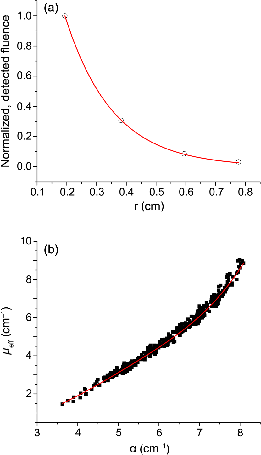$μ_{eff}$ versus $α$ .

This value of $α$ was then converted to $μ_{eff}$ through a simulation library. In order to generate this library, simulations were run at a wide variety of $μ_{eff}$ values. For each simulation of a known $μ_{eff}$ , the value of $α$ was found by fitting Eq. (1) to the simulated data. After this was performed for all simulations, a second-order Fourier series was then fit to the relation between $α$ and $μ_{eff}$ , as shown in Fig. 2(b). The form of this fit was found to be

Eq. (2)

μ_{eff} = a_{0} + a_{1} \cos (| α | w) + b_{1} \sin (| α | w) + a_{2} \cos (2 | α | w) + b_{2} \sin (2 | α | w),

where

a_{0} = 2.49 \times 10^{10}

,

a_{1} = - 3.32 \times 10^{10}

,

b_{1} = - 2.35 \times 10^{8}

,

a_{2} = 8.29 \times 10^{9}

,

b_{2} = 1.18 \times 10^{8}

, and

w = 1.14 \times 10^{- 3}

. The mathematical form of this fit is not of particular scientific interest but was simply used to smooth the data.

Constraining $μ_{eff}$ was required in order to remove ambiguities in the simulation library. In order to directly fit the simulation library to measured data, one would minimize an expression of the form

Eq. (3)

χ^{2} = \sum_{d = 2}^{5} {[φ_{m} (r_{d}) - φ_{MC} (r_{d}, μ_{a}, μ_{s}^{'})]}^{2}

at each wavelength, where

φ_{m}

is the measured, normalized fluence detected at detector position

r_{d}

and

φ_{MC}

is the simulated, normalized fluence detected at detector position

r_{d}

with optical properties

μ_{a}

and

μ_{s}^{'}

. Here,

μ_{s}^{'}

was used due to the relatively employed large source–detector separations. Minimizing Eq. (3), however, results in the scenario were shown in Fig. 3. The gray region in the plot represents combinations of (

μ_{a}

,

μ_{s}^{'}

) that generate a local minimum in Eq. (3). As can be seen, there is no one unique solution to the minimization but a family of equally valid solutions. By inserting the constraint on

μ_{eff}

, we can determine a unique solution to the problem.

Fig. 3

Fitting simulated data to the full simulation library using Eq. (3). The gray region represents local minima in optimization of Eq. (3) and the black region corresponds to values of $μ_{eff}$ that are within 5% of that determined in step 1 of the algorithm. The overlapping portion of the curves is shown filled by horizontal lines.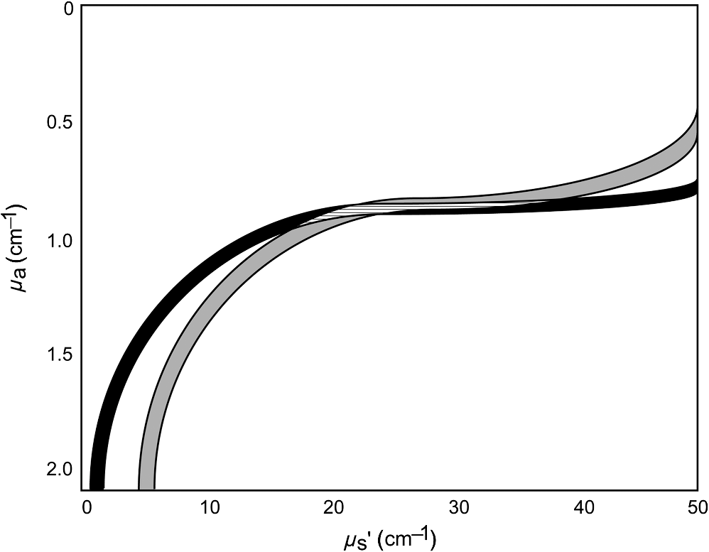

This was done by minimizing Eq. (3) as described previously but only considering entries in the simulation library with a $μ_{eff}$ value within 5% of the $μ_{eff}$ found in step 1 of the fitting algorithm. These $μ_{eff}$ values are shown by the black curve in Fig. 3. Doing so creates a region, composed of the overlapping portion of the black and gray curves shown filled by horizontal lines in Fig. 3, over which we can find the optimum values of absorption and scattering coefficients by minimizing Eq. (3). This results in plots of $χ^{2}$ versus $μ_{a}$ and $χ^{2}$ versus $μ_{s}^{'}$ such as those shown in Fig. 4.

Fig. 4

Determination of (a) $μ_{a}$ and (b) $μ_{s}^{'}$ from constrained minimization of Eq. (3). Open circles represent $χ^{2}$ values for combinations of $μ_{a}$ and $μ_{s}^{'}$ in the simulation library, whereas solid lines represent a seventh-order polynomial fit to these data. The appropriate optical property combination is found by determining the minima in these fits.

For both $μ_{a}$ and $μ_{s}^{'}$ , a seventh-order polynomial was fit to curves, such as those shown in Fig. 4, in order to determine the optimum values of the optical properties. As an error check, these determined values, $μ_{a, fit}$ and $μ_{s, fit}^{'}$ , were used with the value of $μ_{eff}$ from step 1 of the algorithm to calculate

Eq. (4)

μ_{a, calc} = \frac{1}{2} [- μ_{s, fit}^{'} + \sqrt{{(μ_{s, fit}^{'})}^{2} + \frac{4}{3} μ_{eff}^{2}}],

Eq. (5)

μ_{s, calc}^{'} = \frac{μ_{eff}^{2}}{3 μ_{a, fit}} - μ_{a, fit} .

If these calculated values, $μ_{a, calc}$ and $μ_{s, calc}^{'}$ , differed from $μ_{a, fit}$ and $μ_{s, fit}^{'}$ by $> 20 %$ , the data for this wavelength were discarded, and fitting proceeded to the next wavelength. This was done to exclude data for which $μ_{eff}$ was not known well enough to generate curves of comparable quality to those shown in Fig. 4.

The final step of the algorithm involved fitting the values of $μ_{a}$ and $μ_{s}^{'}$ found in step 2 with the known spectral shapes of the absorbers and scatterers present. To do this, the $μ_{s}^{'}$ spectrum was first fit with

Eq. (6)

μ_{s}^{'} (λ) = a {(\frac{λ}{λ_{0}})}^{- b},

where

λ

is the wavelength in nanometers,

λ_{0}

is a fixed normalization wavelength, and

a

and

b

are coefficients in the fit. Here,

λ_{0}

was set to 600 nm. The values of

a

and

b

were constrained to be positive in the fit. Using the

μ_{eff}

spectrum found in step 1 and this fitted

μ_{s}^{'}

spectrum, the

μ_{a}

spectrum was recalculated using Eq. (4). This was done to remove cross-talk between absorption and scattering since the scattering spectrum is known to be smooth. Finally, the absorption spectrum was fit with a superposition of known absorption basis spectra using a nonlinear optimization. Spectral fitting was performed using a constrained nonlinear optimization algorithm (fmincon, MATLAB®, Mathworks, Natick, Massachusetts).

3. Results

Typical spectra collected in a phantom consisting of 1 L of deionized water, 40 mL of Intralipid-20%, and 280 μL of $10 mg / mL$ MnTPPS are shown in Fig. 5. These spectra have been background subtracted and corrected for the effects of system response and fiber throughput, as specified in Sec. 2.

Fig. 5

Measured spectra, corrected for dark background, system response, and fiber throughput, in a phantom consisting of 1 L of deionized water, 40 mL of Intralipid-20%, and 280 μL of $10 mg / mL$ MnTPPS. Broadband white light was delivered by fiber 1 and detected by fibers 2 to 5.

The spectra were then processed using the fitting algorithm described above. In the first step, Eq. (1) was fit to the spatially resolved spectra at each wavelength, as shown in Fig. 6(a). The values of $α$ found at each wavelength were then converted to $μ_{eff}$ , as shown in Fig. 2(b). This resulted in recovered $μ_{eff}$ spectra such as the one shown in Fig. 6(b). The open circles represent fitted $μ_{eff}$ values, and the solid line is the calculated $μ_{eff}$ based on the known optical properties of the phantom. As can be seen, the $μ_{eff}$ spectrum is recovered fairly well, with an average error of 10.3%. The fitted $μ_{eff}$ spectrum tends to overestimate at shorter wavelengths and underestimate at longer wavelengths. This tendency is largely removed in later steps of the fitting process.

Fig. 6

Step 1 of optical property fitting algorithm for a phantom with a MnTPPS concentration of 12.5 μM and an Intralipid-20% concentration of $55 mL / L$ . (a) Fitting of $φ (r)$ with Eq. (1), shown on a log scale, at $λ = 520 nm$ . Open circles represent measured data and the solid black line represents the exponential fit. (b) Recovered $μ_{eff}$ values (open circle) found using the scheme shown in Fig. 2(b). Error bars represent standard deviations over three repeated measurements of the same phantom. The actual $μ_{eff}$ spectrum, shown by the solid red line, is derived from the known concentrations of MnTPPS and Intralipid.

In the second step of the fitting process, the $μ_{eff}$ values found in step 1 were used to constrain a fit to the simulation library given by Eq. (3). This resulted in plots such as those shown in Fig. 4, which were used to find the optical properties at each wavelength. Typical recovered optical property spectra are shown in Fig. 7. In this case, error bars are standard deviations over repeated measurements of the same phantom.

Fig. 7

Recovery of (a) $μ_{a}$ and (b) $μ_{s}'$ from measurements of the tissue-simulating phantom shown in Fig. 6. Fitting was performed by minimization of Eq. (3), constrained by the $μ_{eff}$ spectrum shown in Fig. 6(b). Open circles represent recovered optical properties and the solid lines represent known optical properties of the phantom. Error bars represent standard deviations over three repeated measurements of the same phantom.

In the final step of the fitting algorithm, spectra were fitted with the absorber and scatterer spectral shapes. The results of this are shown in Fig. 8. Here, the open circles represent recovered optical properties and the solid lines represent known optical properties of the phantom. As can be seen, $μ_{a}$ and $μ_{s}^{'}$ are both recovered well, with mean errors of 8.8% and 13.3%, respectively.

Fig. 8

Results of fitting the (a) $μ_{a}$ and (b) $μ_{s}^{'}$ spectra shown in Fig. 7, with the known shape of the absorption spectrum and the known form of the scattering spectrum. Open circles represent recovered optical properties and the solid lines represent known optical properties of the phantom. Error bars represent standard deviations over three repeated measurements of the same phantom.

The results of the three sets of MnTPPS phantom experiments are summarized in Fig. 9. Each experiment corresponds to one particular scatterer concentration, with measurements made at four MnTPPS concentrations, ranging from 12.5 to 50 μM. In Fig. 9(a), data points are averages over all three sets of experiments for the given MnTPPS concentrations, with error bars corresponding to standard deviation. For Fig. 9(b), data points are averages over a particular experiment at a given Intralipid concentration, ranging from 55 to $90 mL / L$ , for all values of MnTPPS concentration. Error bars correspond to standard deviations. As can be seen, the fitting of $μ_{a}$ is consistently good, with a mean error of 9.0% and a maximum error of 38%. The fitting of $μ_{s}^{'}$ is poorer, with a mean error of 19% and a maximum error of 48%.

Fig. 9

Combined results of (a) $μ_{a}$ and (b) $μ_{s}^{'}$ recovery for all three sets of experiments. Data points shown in (a) are averages over measurements made in three phantoms with varying Intralipid concentration, at MnTPPS concentrations of 12.5 μM (open circles), 25 μM (open squares), 37.5 μM (open triangles), and 50 μM (inverse triangles). Solid lines correspond to known absorption spectra for the given MnTPPS concentrations. Data points in (b) correspond to averages over measurements made in three phantoms at Intralipid concentrations of 55 (open circles), 75 (open squares), and $90 mL / L$ (open triangles), at four MnTPPS concentrations. The solid lines represent the known scattering spectrum for each of the three phantoms.

The same procedure was repeated for phantoms containing intact human erythrocytes. Typical fitted $μ_{a}$ spectra are shown in Fig. 10(a) for the case of fully oxygenated and fully deoxygenated hemoglobin phantoms. As can be seen, spectra from both oxy- and deoxyhemoglobin can be recovered from measurements made in phantoms. The algorithm tends to slightly overestimate the absorption of oxyhemoglobin and underestimate the absorption of deoxyhemoglobin.

Fig. 10

(a) Recovered $μ_{a}$ spectra for phantom measurements made in fully oxygenated (open circles) and fully deoxygenated (open squares) hemoglobin. Solid lines represent the known $μ_{a}$ spectra given the known hemoglobin concentration and oxygen saturation. (b) Recovery of ${SO}_{2}$ from measurements made in phantoms containing erythrocytes. Each data point corresponds to a measurement made in a phantom at a particular oxygenation. The solid line represents perfect agreement.

In addition to full oxygenation and deoxygenation, cases in which there are contributions from both oxy- and deoxyhemoglobin are interesting. The ability of the algorithm to separate the contributions of both species of hemoglobin can be assessed by examining the recovery of ${SO}_{2}$

Eq. (7)

{SO}_{2} = \frac{[{HbO}_{2}]}{[Hb] + [{HbO}_{2}]},

where

[{HbO}_{2}]

is the concentration of oxyhemoglobin and

[Hb]

is the concentration of deoxyhemoglobin. This is shown in Fig. 10(b).

{SO}_{2}

values are recovered well, with a mean error of 12% and a maximum error of 73%. As mentioned previously, the algorithm tends to over fit the contribution of oxyhemoglobin, so

{SO}_{2}

values are skewed slightly high in the recovery. This also results in larger errors at smaller values of

{SO}_{2}

, which is the cause of the reported 73% maximum error for fully deoxygenated hemoglobin.

The measured oxygen partial pressure and ${SO}_{2}$ are related through the Hill equation, given by

Eq. (8)

{SO}_{2} = \frac{p O_{2}^{n}}{p O_{2}^{n} + p 50^{n}},

where

p O_{2}

is the measured oxygen partial pressure,

p 50

is the partial pressure at which hemoglobin is 50% saturated, and

n

is a parameter known as the Hill coefficient.¹⁵ Since we obtain

{SO}_{2}

from spectral fitting, we can determine the values of these coefficients by fitting Eq. (8) to the measured data. This is shown for the case of a single phantom in Fig. 11. In this case, the parameters in Eq. (8) were found to be

p 50 = 21.9 torr

and

n = 2.4

. For all phantom measurements combined, these values were found to be

32.3 \pm 10

and

2.3 \pm 0.4 torr

. These values are close to the typical values of

p 50 = 26 torr

and

n = 2.8

although the recovered

p 50

are on average 24% higher than the typical value of 26 torr.¹⁶

Fig. 11

Recovered ${SO}_{2}$ values (open squares) as a function of measured $p O_{2}$ for a single phantom, with the corresponding fit (solid line) obtained using Eq. (8). This fit yielded values of $p 50 = 21.9$ and $n = 2.44$ .

Based on the tracking of photon paths in MC simulations, we found that the volume sampled by spectroscopy was weakly sensitive to the tissue scattering coefficient. For example, with values of $μ_{a} = 0.1 {cm}^{- 1}$ and $μ_{s}^{'} = 20 {cm}^{- 1}$ , 49% of photon packets detected at the fiber adjacent to the source were found to traverse paths further than a radius of 5 mm from the optical probe. When the value of $μ_{s}^{'}$ was decreased to $10 {cm}^{- 1}$ , 54% of photon packets were found to sample this volume. Thus, an increase in reduced scattering coefficient resulted in spectroscopy sampling a region closer to the probe. For $μ_{s}^{'}$ values of 20 and $10 {cm}^{- 1}$ , $\sim 24 %$ and 29% of detected photon packets, respectively, traversed paths that extended to a radius of 7.5 mm from the probe. The effects of changing absorption coefficient were negligible. With $μ_{s}^{'} = 20 {cm}^{- 1}$ , 49% of photon packets detected were found to sample a volume $> 5 mm$ from the optical probe for both $μ_{a} = 0.1$ and $0.2 {cm}^{- 1}$ . The value of the absorption coefficient did not influence the volume sampled by spectroscopy but had a comparatively larger effect on the magnitude of the detected signal.

4. Discussion

Here, we present a method that utilizes a single encapsulated optical probe that is capable of recovering optical properties over a wide range of absorption and scattering coefficients. We have shown the technique to be valid for transport albedos as low as 0.95, which is a larger range than for the diffusion approximation. We have demonstrated recovery of $μ_{a}$ with a mean error of 9% and $μ_{s}^{'}$ recovery with a mean error of 19%, which are comparable to errors found in previous studies of interstitial optical property recovery. Wang and Zhu⁸ demonstrated the recovery of interstitial optical properties using multiple isotropic detectors and a diffusion model. In simulations, they were able to recover $μ_{a}$ with an error of 16% and $μ_{s}^{'}$ with an error of 4%. They reported the recovery of interstitial optical properties in vivo but did not comment on the accuracy of the reconstruction. Chin et al.¹⁷ performed recovery of optical properties using relative interstitial steady-state reflectance measurements. Their method resulted in recovery of optical properties to within $\sim 20 %$ for measurements made in tissue-simulating phantoms containing Intralipid and Naphthol Green. Dimofte et al.¹⁸ also reported a method for the determination of interstitial optical properties using point measurements made in a linear channel at a fixed distance from a point source. Using a diffusion approximation, they demonstrated the recovery of $μ_{a}$ and $μ_{s}^{'}$ with mean errors of 8% and 18%, respectively. The errors we demonstrate for our method are comparable to these values.

A number of studies have also examined optical property recovery in the context of hemoglobin spectroscopy. Here, we demonstrated recovery of ${SO}_{2}$ with an average error of 12% and were able to recover reasonable values for the Hill parameters. Hemoglobin oxygen dynamics have been studied extensively using spatially resolved diffuse reflectance measurements made with surface-contact probes. Previous studies performed in our laboratory have demonstrated accurate recovery of ${SO}_{2}$ and of the parameters in the Hill equation. ¹⁹^,²⁰ Due to the direct applicability of analytical methods to the surface-contact geometry, these studies showed more rigorous recovery of ${SO}_{2}$ and the Hill parameters. In the case of interstitial spectroscopy, there have been fewer quantitative studies done on hemoglobin oxygen dynamics. Thompson et al.²¹ demonstrated interstitial measurements of ${SO}_{2}$ during PDT of nodular basal cell carcinoma, with the value varying widely among patients. However, they do not provide any preclinical evaluation of the accuracy of this recovery. Yu et al.²² also demonstrated interstitial recovery of ${SO}_{2}$ and total hemoglobin concentration during motexafin lutetium PDT of the prostate. They found that both values decreased during PDT. Kruijt et al.²³ described a similar trend in a mouse model during m-tetrahydroxyphenylchlorin PDT using multiple isotropic probes. Most of these techniques require the insertion of multiple spectroscopy fibers, which can be unattractive in certain clinical situations.

Our algorithm is only valid for certain ranges of optical properties. We have not found any limits on the recovery of $μ_{a}$ , but the valid $μ_{s}^{'}$ range only extends over a limited span. This places limits on the values of $μ_{eff}$ that can be recovered due to the dependence of $μ_{eff}$ on $μ_{s}^{'}$ . The relationship between $α$ and $μ_{eff}$ described previously only holds for values of $μ_{s}^{'}$ ranging from $\sim 10$ to $30 {cm}^{- 1}$ . We hypothesize that this limitation is due to the geometry of the probe and the assumptions made in step 1 of the fitting algorithm. Since each of the spectroscopy fibers is in a different position and orientation on the probe, some amount of scattering is required to ensure that adequate signal is detected at each of the fibers. We have determined that the technique presented here requires a transport albedo higher than $\sim 0.95$ , with the experiments presented here having values of $a^{'}$ ranging from 0.94 to 0.998. This allows for recovery of a wider range of optical properties than methods using the diffusion approximation, which generally require a transport albedo of at least 0.98.²⁴ However, other methods such as the $P_{3}$ approximation allow reconstruction of much lower transport albedos.⁵

In addition to the limitation on low scattering coefficients, our method also does not work well for very high scattering coefficients. This is due to the assumption of a single radial separation $r$ between fibers in Eq. (1). At reasonable scattering coefficients, this assumption is valid as photons tend to follow roughly the same path from source to detector. At higher scattering coefficients, photons can readily travel in both directions (i.e., clockwise and counterclockwise) around the probe from source to detector. This results in the same source–detector pair having multiple possible values of $r$ along the surface of the probe, which causes Eq. (1) to be fit poorly.

Some of the error in optical property estimation found in the current scheme may be due to the relatively small number of source–detector separations available with this probe. The six spectroscopy fibers afford five source–detector separations. In practice, we found that only the first four detectors measured any appreciable signal for reasonable integration times. In our previous work with surface-contact diffuse reflectance spectroscopy, five to eight source–detector separations were required for accurate recovery of optical properties.²⁵ The limited number of spectroscopy fibers in the probe, therefore, necessitates additional processing, places potential limits on the accuracy of optical property recovery, and motivates the design of future optical probes.

Much of the time, we wish to know the optical properties of tissue so that we can determine the light dose that will be delivered to this tissue by a given iPDT treatment. It is, therefore, important to consider the effects that the error in recovered optical properties will have on the expected fluence distribution in tissue. To examine this, we consider the case of a 2-cm cylindrical diffusing fiber delivering a light dose of $100 J / cm$ embedded in tumor tissue with $μ_{a} = 0.2 {cm}^{- 1}$ and $μ_{s}^{'} = 10 {cm}^{- 1}$ . For the true optical properties, MC simulations show that the delivered light dose at a radial distance of 5 mm from the center of the diffuser will be $115 J / {cm}^{2}$ . If we introduce errors in $μ_{a}$ and $μ_{s}^{'}$ similar to those obtainable by our method, this value is changed to $110 J / {cm}^{2}$ . Therefore, a 9% error in $μ_{a}$ and a 19% error in $μ_{s}^{'}$ lead to a 4% error in estimates of light dose at 5 mm.

Acknowledgments

This work was supported by NIH grant CA68409 and a Research and Innovation Grant from the University of Rochester.

References

1.

T. J. FarrellM. S. PattersonB. Wilson, “A diffusion theory model of spatially resolved, steady-state diffuse reflectance for the noninvasive determination of tissue optical properties in vivo,” Med. Phys., 19 (4), 879 –888 (1992). http://dx.doi.org/10.1118/1.596777 MPHYA6 0094-2405 Google Scholar

2.

Q. Wanget al., “Broadband ultraviolet-visible optical property measurement in layered turbid media,” Biomed. Opt. Express, 3 (6), 1226 –1240 (2012). http://dx.doi.org/10.1364/BOE.3.001226 BOEICL 2156-7085 Google Scholar

3.

N. RajaramT. H. NguyenJ. W. Tunnell, “Lookup table-based inverse model for determining optical properties of turbid media,” J. Biomed. Opt., 13 (5), 050501 (2008). http://dx.doi.org/10.1117/1.2981797 JBOPFO 1083-3668 Google Scholar

4.

M. G. NicholsE. L. HullT. H. Foster, “Design and testing of a white-light, steady-state diffuse reflectance spectrometer for determination of optical properties of highly scattering systems,” Appl. Opt., 36 (1), 93 –104 (1997). http://dx.doi.org/10.1364/AO.36.000093 APOPAI 0003-6935 Google Scholar

5.

E. L. HullT. H. Foster, “Steady-state reflectance spectroscopy in the P3 approximation,” J. Opt. Soc. Am. A, 18 (3), 584 –599 (2001). http://dx.doi.org/10.1364/JOSAA.18.000584 JOAOD6 0740-3232 Google Scholar

6.

J. C. FinlayT. H. Foster, “Hemoglobin oxygen saturations in phantoms and in vivo from measurements of steady-state diffuse reflectance at a single, short source-detector separation,” Med. Phys., 31 (7), 1949 –1959 (2004). http://dx.doi.org/10.1118/1.1760188 MPHYA6 0094-2405 Google Scholar

7.

S. FengF.-A. ZengB. Chance, “Photon migration in the presence of a single defect: a perturbation analysis,” Appl. Opt., 34 (19), 3826 –3837 (1995). http://dx.doi.org/10.1364/AO.34.003826 APOPAI 0003-6935 Google Scholar

8.

K. K.-H. WangT. C. Zhu, “Reconstruction of in-vivo optical properties for human prostate using interstitial diffuse optical tomography,” Opt. Express, 17 (14), 11665 –11672 (2009). http://dx.doi.org/10.1364/OE.17.011665 OPEXFF 1094-4087 Google Scholar

9.

P. R. Bargoet al., “In vivo determination of optical properties of normal and tumor tissue with white light reflectance and an empirical light transport model during endoscopy,” J. Biomed. Opt., 10 (3), 034018 (2005). http://dx.doi.org/10.1117/1.1921907 JBOPFO 1083-3668 Google Scholar

10.

P. Agostiniset al., “Photodynamic therapy of cancer: an update,” CA Cancer J. Clin., 61 (4), 250 –281 (2011). http://dx.doi.org/10.3322/caac.v61:4 CAMCAM 0007-9235 Google Scholar

11.

H. J. van Staverenet al., “Light scattering in Intralipid-10% in the wavelength range of 400–1100 nm,” Appl. Opt., 30 (31), 4507 –4514 (1991). http://dx.doi.org/10.1364/AO.30.004507 APOPAI 0003-6935 Google Scholar

12.

T. M. BaranT. H. Foster, “New Monte Carlo model of cylindrical diffusing fibers illustrates axially heterogeneous fluorescence detection: simulation and experimental validation,” J. Biomed. Opt., 16 (8), 085003 (2011). http://dx.doi.org/10.1117/1.3613920 JBOPFO 1083-3668 Google Scholar

13.

L. WangS. L. JacquesL. Zheng, “MCML—Monte Carlo modeling of light transport in multi-layered tissues,” Comput. Methods Programs Biomed., 47 (2), 131 –146 (1995). http://dx.doi.org/10.1016/0169-2607(95)01640-F CMPBEK 0169-2607 Google Scholar

14.

S. Prahl, “Optical absorption of hemoglobin,” (2013) http://omlc.ogi.edu/spectra/hemoglobin/ January ). 2013). Google Scholar

15.

W. E. L. BrownA. V. Hill, “The oxygen-dissociation curve of blood, and its thermodynamical basis,” Proc. R. Soc. Lond., 94 297 –334 (1923). http://dx.doi.org/10.1098/rspb.1923.0006 PRSLAZ 0370-1662 Google Scholar

16.

L. Stryer, Biochemistry, W. H. Freeman and Company, New York (1988). Google Scholar

17.

L. C. L. Chinet al., “Determination of the optical properties of turbid media using relative interstitial radiance measurements: Monte Carlo study, experimental validation, and sensitivity analysis,” J. Biomed. Opt., 12 (6), 064027 (2007). http://dx.doi.org/10.1117/1.2821406 JBOPFO 1083-3668 Google Scholar

18.

A. DimofteJ. C. FinlayT. C. Zhu, “A method for determination of the absorption and scattering properties interstitially in turbid media,” Phys. Med. Biol., 50 2291 –2311 (2005). http://dx.doi.org/10.1088/0031-9155/50/10/008 PHMBA7 0031-9155 Google Scholar

19.

E. L. HullM. G. NicholsT. H. Foster, “Quantitative broadband near-infrared spectroscopy of tissue-simulating phantoms containing erythrocytes,” Phys. Med. Biol., 43 3381 –3404 (1998). http://dx.doi.org/10.1088/0031-9155/43/11/014 PHMBA7 0031-9155 Google Scholar

20.

J. C. FinlayT. H. Foster, “Recovery of hemoglobin oxygen saturation and intrinsic fluorescence with a forward-adjoint model,” Appl. Opt., 44 (10), 1917 –1933 (2005). http://dx.doi.org/10.1364/AO.44.001917 APOPAI 0003-6935 Google Scholar

21.

M. S. Thompsonet al, “Clinical system for interstitial photodynamic therapy with combined on-line dosimetry measurements,” Appl. Opt., 44 (19), 4023 –4031 (2005). http://dx.doi.org/10.1364/AO.44.004023 APOPAI 0003-6935 Google Scholar

22.

G. Yuet al., “Real-time in situ monitoring of human prostate photodynamic therapy with diffuse light,” Photochem. Photobiol., 82 1279 –1284 (2006). http://dx.doi.org/10.1562/2005-10-19-RA-721 PHCBAP 0031-8655 Google Scholar

23.

B. Kruijtet al., “Monitoring interstitial m-THPC-PDT in vivo using fluorescence and reflectance spectroscopy,” Lasers Surg. Med., 41 653 –664 (2009). http://dx.doi.org/10.1002/lsm.v41:9 LSMEDI 0196-8092 Google Scholar

24.

J. B. Fishkinet al., “Gigahertz photon density waves in a turbid medium: theory and experiments,” Phys. Rev. E, 53 (3), 2307 –2319 (1996). http://dx.doi.org/10.1103/PhysRevE.53.2307 PLEEE8 1063-651X Google Scholar

25.

T. M. Baranet al., “Optical property measurements establish the feasibility of photodynamic therapy as a minimally invasive intervention for tumor of the kidney,” J. Biomed. Opt., 17 (9), 098002 (2012). http://dx.doi.org/10.1117/1.JBO.17.9.098002 JBOPFO 1083-3668 Google Scholar

Citation Download Citation

Timothy M. Baran, Michael C. Fenn, and Thomas H. Foster "Determination of optical properties by interstitial white light spectroscopy using a custom fiber optic probe," Journal of Biomedical Optics 18(10), 107007 (22 October 2013). https://doi.org/10.1117/1.JBO.18.10.107007

Published: 22 October 2013

Access the abstract

JOURNAL ARTICLE
10 PAGES

DOWNLOAD PAPER SAVE TO MY LIBRARY

GET CITATION

CITATIONS

Cited by 14 scholarly publications.

Explore citations on Lens.org

RIGHTS & PERMISSIONS

Get copyright permission Get copyright permission on Copyright Marketplace

KEYWORDS

Optical properties

Spectroscopy

Scattering

Absorption

Sensors

Tissue optics

Solids

1.

Introduction

2.

Materials and Methods

2.1.

Probe Design and Monte Carlo Model

Fig. 1

2.2.

Phantom Preparation

2.3.

Data Collection and Correction

2.4.

Optical Property Recovery Algorithm

Eq. (1)

Fig. 2

Eq. (2)

Eq. (3)

Fig. 3

Fig. 4

Eq. (4)

Eq. (5)

Eq. (6)

3.

Results

Fig. 5

Fig. 6

Fig. 7

Fig. 8

Fig. 9

Fig. 10

Eq. (7)

Eq. (8)

Fig. 11

4.

Discussion

Acknowledgments

References

Show All Keywords

Keywords/Phrases

Search In:

Publication Years