Tracking mechanical wave propagation within tissue using phase-sensitive optical coherence tomography: motion artifact and its compensation

Shaozhen Song; Zhihong Huang; Ruikang K. Wang

doi:10.1117/1.JBO.18.12.121505

22 October 2013 Tracking mechanical wave propagation within tissue using phase-sensitive optical coherence tomography: motion artifact and its compensation

Shaozhen Song, Zhihong Huang, Ruikang K. Wang

Author Affiliations +

Journal of Biomedical Optics, Vol. 18, Issue 12, 121505 (October 2013). https://doi.org/10.1117/1.JBO.18.12.121505

Abstract

We describe theoretical and experimental investigations of motion artifacts that can arise in the detection of shear wave propagating within tissue with phase-sensitive optical coherence tomography. We find that the motion artifact is a combined product of sample surface motion and refractive index difference between sample and air, which cannot be neglected when estimating the tissue motion within tissue. A method of compensating the motion artifact is demonstrated, the results of which emphasize the need for surface motion compensation when measuring the mechanical response for elastography or other biomedical applications.

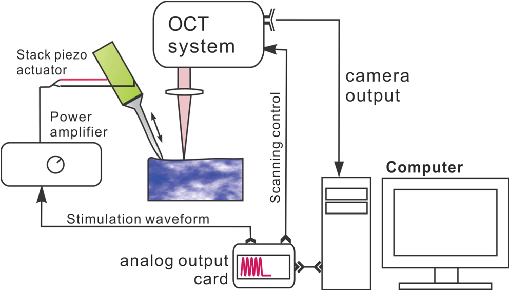
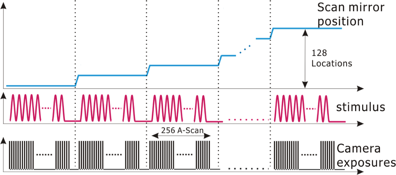
1. Introduction

Since it was reported on in 1991,¹ optical coherence tomography (OCT) has gradually become the tool of choice for noninvasive three-dimensional imaging of biological and industrial samples.² Particularly important is its unique combination of noninvasive, noncontact, high spatial resolution, high sensitivity, and high speed, the features that have attracted increased interest in a wide range of preclinical and clinical applications, for example, in ophthalmology, cardiology, neurology, dermatology, etc.³ Traditionally, OCT is used for imaging tissue morphology. However, one of the recent developments has been in the use of OCT for high sensitive detection of tissue microscopic motion/deformation in vivo. Because the tissue motion is directly related to its biomechanical properties, the monitoring and imaging of this motion provides important information about tissue mechanical compliance.

The first report that used OCT to detect tissue micro-deformation was demonstrated under external compression load by Schmitt in 1998,⁴ introducing the term of OCT elastography (OCE). Since then, various techniques were augmented to OCT for the purpose of tracking tissue motion. In the early development of OCE, the method was based on a straightforward approach that employs intensity-based speckle tracking to provide tissue displacement under static or quasi-static mechanical load.⁵^–⁷ However, the intrinsic limitations of the traditional speckle tracking algorithm make this method difficult to provide accurate quantitative elastography, largely due to speckle intensity and shape variations.⁸

To mitigate the problems in the use of speckle tracking, the phase information intrinsically available in the complex OCT signals has been explored to accurately measure minute tissue motion with high sensitivity down to a subnanometer scale.⁹^–¹¹ Thanks to the rapid development of Fourier domain OCT that significantly improved the image acquisition speed and sensitivity, it is now possible to measure and/or image the minute dynamic tissue motion in real time, making an important step toward in vivo applications. In this regard, increased attention has been paid to the use of OCT to track and monitor mechanical waves propagating within tissue, induced by either external¹² or internal¹³ mechanical stimuli. The methods of external stimuli include the use of acoustic radiation force¹⁴ or simply by a contact mechanical vibrator.¹²^,¹⁵ Recently, we introduced the use of phase-sensitive OCT (PhS-OCT) to sensitively detect surface acoustic waves (SAW) propagating on skin¹⁶ and cornea¹⁷ surfaces, leading to quantification of the elasticity of underlying tissues. Others have used PhS-OCT to detect the shear wave¹⁸^,¹⁹ and longitudinal wave.²⁰ The assumption here is that the phase changes detected by PhS-OCT represent the true localized motion within tissue. While this is true in the detection of blood flow velocity,²¹^,²² we notice that the detected phase changes do not accurately represent the localized tissue motion, particularly when detecting the induced shear waves within tissue, leading to the measurements being severely contaminated by a motion artifact.

Image artifacts have been an important topic of research in nearly all medical imaging modalities because they may degrade image quality and cause inaccurate clinical interpretation of images. Artifacts in motion detection are even more critical in OCE because the error in the detected mechanical responses could lead to inaccurate inversion results of tissue elasticity.

The purpose of this paper is to describe the theoretical and experimental investigations of artifacts that can arise in the motion detection with PhS-OCT when mechanical stimulation is applied on sample surface or surface motion is induced unintentionally. While spectral-domain OCT (SD-OCT)²³^,²⁴ and swept source OCT (SS-OCT)²⁵^,²⁶ are based on similar spectral interferometric principles and can be used to detect motion using phase-resolved approach, the motion signal from these techniques could be contaminated by similar artifacts. We present the results that provide an understanding of the motion artifacts when detecting the tissue motion in the underlying structures. An effective method of compensating for the motion artifacts is proposed and demonstrated. The results emphasize the need for surface motion compensation when measuring the mechanical response for elastography or other biomedical applications related to tissue motion detection.

2. Theoretical Aspects

2.1.

Phase-Resolved OCT Motion Detection

Figure 1(a) shows the schematic of a basic configuration of an SD-OCT system. A broadband light is used as the illumination source, which is split into reference beam and sample beam. Reference beam is delivered to a stationary mirror, while sample beam is focused onto the specimen. The coupler recombines the backscattered light from both reference and sample arms to form a spectral interferogram, which is subsequently detected by a line-scan camera-based spectrometer. Hence, each pixel on the CCD array detects optical power as a function of optical wavenumber, $k$ .

Fig. 1

Schematic of system for shear wave imaging.

Optical frequency-domain imaging is accomplished with a swept frequency laser source, thus also termed as SS-OCT.²⁶ As shown in Fig. 1(b), SS-OCT differs from SD-OCT in the light source used and the interference detection method, in which the reflected lights from reference mirror and sample pass through two circulators and recombine by a $2 \times 2$ coupler before being detected by a balanced photodetector.

The photocurrent associated with the interference fringes at the detector can be expressed by²⁷

Eq. (1)

i (k) = \frac{1}{2} ρ S (k) δ k {R_{R} + \sum_{n} R_{n} + 2 \sqrt{R_{R}} \sum_{n} \sqrt{R_{n}} \cos [2 k (Δ z_{n} + δ z_{n})]},

where

S (k)

is the source power spectral density;

k

is the wave number (in radians per meter);

δ k

is the spectral bandwidth of light source;

ρ

is the detector responsivity;

R_{R}

is the reference arm reflectivity; and

R_{n}

is the reflectivity of the sample at location

z_{n}

(i.e., local reflector).

Δ z_{n}

is an integer multiple of discrete sampling interval in

z

domain (depth), given by

m π / δ k

, where

m

is any positive or negative integer indexing one-dimensional

z

domain A-scan array.

δ z_{n}

is the subresolution deviation of the local reflector (scatterer) location away from

Δ z_{n}

. As the PhS-OCT mainly detects the subresolution movement,

δ z_{n}

is the primary determinant factor of the OCT signal phase.

In the case of SD-OCT, $i (k)$ is the integration over A-scan exposure time, while in SS-OCT, $i (k)$ is instantly sampled by a high-speed photodetector. For either case, a Fourier transformation of $i (k)$ (realistically, discrete Fourier transformation) will give the complex-valued $z$ domain signal.²⁷

Eq. (2)

I (2 Δ z_{n}) = \frac{ρ S_{0} {(R_{R} R_{n})}^{1 / 2}}{2 e f_{s}} E (2 δ z_{n}) \exp (j k_{0} 2 δ z_{n}),

where

S_{0}

is the total sample illumination power, i.e.,

\int S (k) d k

. The term

E (2 δ z_{n})

denotes the unity-amplitude

z

domain autocorrelation function,

k_{0}

is source center wavenumber, and

f_{s}

is the A-scan rate in Hertz. Note that the noise term is not included in the expression of complex-valued intensity signal because the phase sensitivity is not the focus of this paper. For simplicity, the contribution from multiple scattering is neglected in this equation.

As seen in Eq. (2), the phase of $I (2 Δ z_{n})$ is proportional to $δ z_{n}$ . Hence, the difference in optical path length (OPL), i.e., the difference in $δ z_{n}$ , can be calculated from the phase difference of the complex signals in the $z$ domain. For the phase-resolved method,²⁸ the instantaneous displacement of a local scatterer between two successive A-scans is equivalent to the instantaneous Doppler shift represented by the derivative of the phase with respect to time, which can be written as

Eq. (3)

d (t) = \frac{λ_{0}}{2 \cos θ} f_{dopp} = \frac{λ_{0}}{4 π \cos θ} f_{s} [∠ I (2 Δ z_{n}, t) - ∠ I (2 Δ z_{n}, t - f_{s}^{- 1})] .

Here $∠$ denotes phase operator, $λ_{0}$ is the central wavelength of the light source, $f_{dopp}$ is the Doppler frequency shift, $f_{s}$ is the A-scan rate, and $θ$ is the Doppler angle between optical axis and motion direction. In most cases, one assumes the sample displacement is only in optical axial direction, meaning that only displacement vector projection in the axial direction is detected; Eq. (3) can be simplified to

Eq. (4)

d (z, t) = Δ ϕ (z, t) λ_{0} {(4 π T_{s})}^{- 1},

where

Δ ϕ (z, t)

is the phase difference between adjacent A-scans at location (depth)

z

and time

t

.

2.2.

Artifacts Induced by Air Interface Motion

Currently, the use of PhS-OCT often assumes that $Δ ϕ (z, t)$ evaluated between adjacent A-scans is caused by the displacement of the scatterer at the location $z$ . However, OCT phase signal is in fact only sensitive to the path-length difference between the OPL of reference mirror and the OPL of the scatterer at the location $z$ in the interferometer. In terms of measured phase change, it is accumulated over the optical path along the sample beam. Thus, $Δ ϕ (z, t)$ is the true representation of the displacement of the scatterer only when there is no OPL perturbation above the scatterer of interest. This requirement is met when (1) there is no tissue movement above the scatterer and (2) refractive index along the beam propagating path in the sample arm is uniform over time. While these conditions are generally satisfied in the use of phase-resolved technique to evaluate the blood flow velocity, they become complicated when using PhS-OCT to monitor/trace the propagating waves within sample induced by a mechanical stimulus. Mechanical stimulus may induce different mechanical waves propagating within tissue, for example, shear wave, Rayleigh wave (surface acoustic waves), and longitudinal waves. Even more complicated is the case of heterogeneous properties of the sample because, by definition, elastic heterogeneities produce reflected waves. All these mechanical waves would affect the accuracy of PhS-OCT monitoring of the movement of the scatterer at the location $z$ due to the dynamic mechanical wave of interest.

In the current study, where we are interested in using PhS-OCT to track the shear wave propagating within tissue, the phase difference detected is induced by dynamic OPL change. Assuming that the tissue is uniform in refractive index, two main factors can cause a change in OPL: (1) the motion of the scatterer due to the shear wave of interest and (2) the tissue surface motion at air–tissue interface that perturbs the OPL along the detection beam. The latter becomes a severe artifact in the dynamic motion detection. Because the phase change is accumulated along the optical path, the detected value is the summation of phase changes due to these two motions. This situation is shown in Fig. 2.

Fig. 2

Illustration of a situation when optical coherence tomography (OCT phase) is influenced by both sample surface motion and scatterer motion.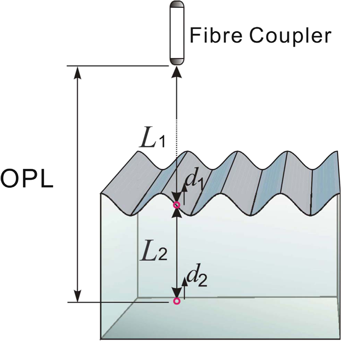

Note that in our case, we did not consider the change of refractive index due to compression wave for two reasons: (1) The change of refractive index caused by compression is very small. Even in an extreme condition of 1% density change under shock compression,²⁹ the refractive index change is only $1.7 \times 10^{- 4}$ . This magnitude is too small to cancel out the OPL change in our study. (2) For gels and soft tissues, the assumption of incompressibility is widely used for modeling mechanical waves in tissue,³⁰^,³¹ where the wave amplitude is small (micron scale).

Assume that the scatterer of interest is located at the depth of $L_{2}$ away from the sample surface, and the distance is $L_{1}$ between sample surface and the fiber coupler where the reference beam and reflected sample beam interfere; the total equivalent OPL is then

Eq. (5)

{OPL}_{0} = L_{1} n_{1} + L_{2} n_{2}

at the time

t = 0

when there is no motion. Here,

n_{1}

is the refraction index of air and

n_{2}

is that of the sample. At a successive A-scan (

t = T_{S}

, where

1 / T_{S}

is the A-scan rate of the OCT system), the sample surface moves a distance of

d_{1}

, while the scatterer travels a distance of

d_{2}

(defining the motion toward detector is positive direction). Thus, the equivalent OPL at the time

t = T_{S}

becomes

Eq. (6)

{OPL}_{1} = (L_{1} - d_{1}) n_{1} + (L_{2} + d_{1} - d_{2}) n_{2} .

The OPL difference between the times $t = 0$ and $t = T_{S}$ , which gives rise to $Δ ϕ$ , is then

Eq. (7)

Δ OPL = {OPL}_{0} - {OPL}_{1} = d_{2} n_{2} + (n_{1} - n_{2}) d_{1} .

Here, the term $d_{2} n_{2}$ is caused by the true motion of the localized scatterer. $(n_{1} - n_{2}) d_{1}$ is caused by the surface motion, e.g., SAW induced by the mechanical stimulus. This latter term would give rise to an artifact to the experimental measurements of the motions beneath the sample surface in the $z$ domain. Therefore, within the B-frame image of the displacement field that is determined by the PhS-OCT system, a propagating surface wave will lead to stripe artifacts according to the above analysis.

From Eq. (7), when the scatterer is close to surface, i.e., $L_{2} \to 0$ , the scatterer displacement will approach the surface displacement, i.e., $\lim_{L_{2} \to 0} d_{2} = d_{1}$ . Then, we have

Eq. (8)

\lim_{L_{2} \to 0} Δ OPL = d_{2} n_{2} + (n_{1} - n_{2}) d_{1} = d_{1} n_{2} + (n_{1} - n_{2}) d_{1} = d_{1} n_{1} .

Thus, if the detected phase near the sample surface is $Δ ϕ_{surf} (z_{surf}, t)$ , we have

Eq. (9)

d_{1} = Δ ϕ_{surf} (z_{surf}, t) / n_{1} .

Therefore, combining Eqs. (9), (7), and (4), the real phase change $Δ ϕ_{c}$ due to the motion of the scatterer at the location $z$ can be deduced.

Eq. (10)

Δ ϕ_{c} (z, t) = Δ ϕ_{d} (z, t) + (n_{2} - n_{1}) Δ ϕ_{surf} (t),

where

Δ ϕ_{d}

and

Δ ϕ_{surf}

are the phase changes directly determined by PhS-OCT at the location

z

and at the surface, respectively.

3. Methods

3.1.

Experimental Setup

In this study, a PhS-OCT system based on SD-OCT configuration was used to observe the artifacts and validate the proposed phase compensation approach. The light source was a superluminescent diode (SLD) (DenseLight Semiconductors Ltd., Singapore) emitting 1.31 μm central wavelength laser with $\sim 46 nm$ spectral bandwidth. The spectrometer consisted of a diffraction grating, focusing lens, and InGaAs line scan camera (Sensors Ltd., USA) with 1024 pixels and 14-bit precision. The imaging was accomplished by a galvo-scanner that scanned the probe beam over the sample. The synchronization among galvo-scanner, mechanical wave generation, and data acquisition was controlled precisely by a house-developed LabVIEW program.

A low-voltage, stacked piezoelectric actuator (Thorlabs, New Jersey) was used to generate mechanical waves propagating in the sample. A power amplifier (AE Techron, Indiana) with a controllable voltage gain was used to optimally drive the actuator’s capacitance. A slender stainless steel rod with a small polished tip was fixed to the actuator as the contact to the sample. The actuator assembly was then mounted to a precision positioning stage, enabling precise advancement of the actuator-tip to gently contact to the sample surface (see Fig. 3).

Fig. 3

Mechanical wave measurement setup.

3.2.

Phantom Preparation

Similar to our previous studies,³² we used tissue-mimicking phantoms to verify our proposed approach. Agar is an easily accessible material that can be used to produce tissue phantoms with controllable mechanical properties similar to those of human soft tissue.³³ To produce these phantoms, a proper amount of agar-agar powder (Fisher Scientific Inc., USA) was stirred into boiling distilled water until completely dissolved. A few drops of milk were added as scattering particles to facilitate OCT detection.

3.3.

Scan Protocol and Reconstruction of Displacement Field

To track shear waves propagating in tissue, the PhS-OCT was operated in M-B mode, wherein a sequence of 256 A-scans (one M-scan) was captured at every spatial location sequentially within the B-scan (total 128 locations) mode while the actuator repeatedly fired the stimulus. Thus, a complete M-B scan consisted of $256 \times 128$ A-scans. The timing of the M-B scan protocol is shown in Fig. 4. The system A-scan rate was set to 46.992 kHz, while M-scan repetition rate was 140 Hz. Each M-B scan acquisition takes $\sim 1 s$ . The 128 M-B scans were rearranged to form 256 B-M scans. In this way, the rearranged B-M scan had an equivalent frame rate the same as the A-line rate ( $\sim 47 kHz$ ). This high frame rate could provide a direct visualization of the propagating mechanical waves within a range of 1 to 7 kHz, commonly with wavelength of 0.1 to 1 mm in soft tissue, which is appropriate for OCT imaging.

Fig. 4

Timing schematic of scanning protocol.

To obtain the displacement field in each frame, the commonly used phase-resolve method was adopted. Before the Fourier transformation, the spectral interferograms data were resampled into the k space evenly distributed,³⁴ and then the depth-resolved phase data were extracted from the complex OCT signals.⁹ Localized motion was determined by evaluating the phase differences between adjacent A-scans within the M-scan [see Eqs. (4) and (10)]. The operation was repeated for all M-scans, and displacement at a given pixel over time was obtained, i.e., $d (x, z, t)$ , assuming $x$ and $z$ are lateral and depth positions, respectively.

3.4.

Modeling of Surface and Shear Wave Pattern

To verify the displacement field in the phantoms, we performed a simulation based on a finite difference model to provide theoretical waveforms for comparison with the artifact-contaminated images. Solutions to wave propagation problems by finite-difference methods (FDM) have been widely used in seismology (e.g., Ref. 35) and biomedical ultrasound (e.g., Ref. 36) for forward modeling the elastic waves, because of their ability to accurately predict the wave propagation in homogeneous media. In this investigation, we adopted an FDM model with the second-order temporal and fourth-order spatial approximations.³⁷ The setup for the simulation model is shown in Fig. 5.

Fig. 5

Model setup for finite difference simulation. Free surface is denoted by $Γ 1$ . $Γ 2$ to $Γ 4$ are fixed boundary. The grid size is scaled for this figure.

Consider the propagation of elastic waves in a Cartesian coordinate system (the $x - z$ system shown in Fig. 5) without external forces; the governing equations of elastic waves take the form³⁷

Eq. (11)

ρ \frac{\partial^{2} u}{\partial t^{2}} = \frac{\partial}{\partial x} [(λ + 2 μ) \frac{\partial u}{\partial x} + λ \frac{\partial v}{\partial z}] + \frac{\partial}{\partial z} [μ (\frac{\partial v}{\partial z} + \frac{\partial u}{\partial x})] ρ \frac{\partial^{2} u}{\partial t^{2}} = \frac{\partial}{\partial x} [μ (\frac{\partial v}{\partial z} + \frac{\partial u}{\partial x})] + \frac{\partial}{\partial z} [(λ + 2 μ) \frac{\partial v}{\partial z} + λ \frac{\partial u}{\partial x}],

where

u

and

v

are the velocity components in

x

and

z

directions; the Lame parameters,

λ

and

μ

, and density,

ρ

, are set to be uniform in the simulation domain. The difference equations are solved for the independent variables on a discrete grid. A detailed numerical solution description can be found in Ref. 37.

On the free surface ( $Γ_{1}$ ), we impose the boundary conditions of

Eq. (12)

[\begin{matrix} (2 μ + λ) \frac{\partial u}{\partial x} + λ \frac{\partial u}{\partial z} & μ (\frac{\partial v}{\partial x} + \frac{\partial u}{\partial z}) \\ μ (\frac{\partial v}{\partial x} + \frac{\partial u}{\partial z}) & (2 μ + λ) \frac{\partial v}{\partial z} + λ \frac{\partial u}{\partial x} \end{matrix}] [\begin{matrix} n_{x} \\ n_{z} \end{matrix}] = 0 .

Here, ${[n_{x}, n_{z}]}^{T}$ is the inward normal of $Γ_{1}$ . Model grid size and time step size are determined by the numerically stable requirement of the FDM. The model is set as a square of $20 \times 20 mm$ with the model grid size at $\sim 12.7 μ m$ and the fixed time step at 10 μs. The simulation was implemented with MATLAB code, from which the snapshots of wave field as a time sequence were obtained.

4. Results

4.1.

Presence of Artifact

To demonstrate the presence of the artifact, a layered glass plate phantom is fabricated to create a circumstance that mechanical wave is propagating within a layer of soft phantom between a free surface and a glass plate, while at the bottom there is an air gap above the substrate rigid body (steel plate), see Fig. 6(a). With this configuration, the steel plate can be safely assumed to be static, i.e., without mechanical waves propagating in it, because the glass plate and a layer of air isolate the acoustic waves from the soft phantom. And also the stimulation is not able to launch detectable motion in steel with given frequency and amplitude. In the experiments, the stimulation tip was driven by a stack piezoelectric actuator, and the tip was emitting 5 kHz sine waves of 5 cycles. All the phantoms were $> 50 mm$ in diameter and at least 15 mm deep, to avoid any reflected wave from the boundaries. The vibration amplitude was $< 3 μ m$ . The tip was a wedge-like shape, with a width of 1.7 mm edge. The waves generated by this tip can therefore be considered approximately planar, having negligible out-of-plane displacement, which simplifies the experiments for two-dimensional analysis. When attaching the tip to the sample, the OCT system was used to provide the real-time B-scan of the region of interest.

Fig. 6

Illustration of phantom configuration. (a) Thin phantom plate. (b) Large homogeous phantom in air. (c) Large homogeous phantom with a layer of oil and a glass plate in the top. Note in (b) and (c), the dashed box indicating imaging range (B-scan) is not in scale.

After processing PhS-OCT data, a video that provides visualization of the propagating mechanical wave was generated. The phase map was encoded with bipolar color map, where red color denotes the motion toward the OCT light beam. The phase image was then overlaid onto the OCT B-scan structural image, with higher transparency for lower amplitude of motion, as shown in Fig. 7. Before mapping the phase, a mask was applied to the phase image. The mask was generated from the structural image so that any pixel with low OCT signal intensity, e.g., from transparent structures, was masked out. This masking method was applied to all the phase images in this paper. Four snapshots of the dynamic wave (displacement field) are shown in Figs. 7(a1) to 7(a4); each snapshot is noted by the time offset from $t = 0$ . The same applies to all the snapshot images in this paper. The bright line at the bottom of each image is the surface of steel plate. The phase artifacts are clearly indicated in these images, with smaller but opposite phase values to the surface phase, as indicated by arrows in Fig. 7. This supports the analyses presented in Sec. 2.2 that a positive phase on a surface will cause a negative phase (artifact) at all locations underneath the surface. Hence, on the B-scan image, the stripe artifacts are created by the surface motion.

Fig. 7

(a1) to (a4) Phase-sensitive OCT (PhS-OCT) detected displacement field [(a1) $t = 5 Ts$ , (a2) $t = 10 Ts$ , (a3) $t = 15 Ts$ , (a4) $t = 20 Ts$ ; $Ts = sampling period$ ]. (b1) to (b4) Compensated displacement fields. Same colorbar as shown in (a1) applies to each subfigure.

The phase compensation method was then applied on these wave field dataset. The results are shown in Figs. 7(b1) to 7(b4). After compensation, the phase artifacts on the steel plate and also on the glass plate surface are eliminated. Corrections to the wave pattern propagating within tissue phantom are also observed, with the amplitude diminishing to zero from surface to bottom. Note that in this figure, there still exists phase signal (red or blue) within some region that is of low OCT signal. This is largely due to the imperfection of the masking method used. This, however, does not affect the demonstration of artifact compensation.

To show the strength of artifact, the displacement waveform at different depths are plotted in Fig. 8, where the compensated and uncompensated waveform at three depths/locations [marked as “+” in Fig. 7(a1)] are given. At depth #1, the vibration amplitude is the largest because this location is close to the phantom surface where the artifact effect is less obvious. As the depth goes deeper to depth #2, both the phase and amplitude show a severe distortion. Because in the deeper region the true displacement becomes smaller while the artifact amplitude is uniform at all depths, the error rate increases significantly at the deeper region. As shown at the bottom pair of waveforms, there is no displacement signal on the steel plate after compensation as expected, demonstrating the effectiveness of the compensation method. Note that the artifact could lead to the increase or decrease of the apparent amplitude (see depth 2 and steel plate) depending on whether it impacts on the true displacement positively or negatively. In the case of “Phantom depth 2,” the artifact has negative effect; therefore, the compensated curve is higher in magnitude than the measured curve.

Fig. 8

Displacement waveforms at three depths of the layered phantom.

4.2.

Wave Field Simulation

As the simulation was intended to create a numerical solution to the wave field in a homogeous phantom, the dimensions and physical parameters were set to mimick the soft phantom. The longitudinal wave (P-wave) and shear wave (S-wave) velocity were set to 1050 and $2.5 m / s$ . The simulation modeled a homogeous phantom with a stimulation source emitting 3 cycles of 5 kHz sine waves on surface. A snapshot of displacement field ( $z$ direction component) is presented in Fig. 9(a). In this figure, to avoid any reflections, only a $2 \times 3.5 mm$ section is shown, which is relatively far from any fixed boundaries. Figure 9(b) is the measured wave propagating pattern at the same time instance of the stimulation. As the stimulation in the experiment was applied with a small angle, the wave front observed in the stimulation presents some difference from that in the simulation. In general, the wavelength, amplitude, and the wave pattern reached good agreements between the experiment and the simulation.

Fig. 9

A snapshot of displacement field from the numerical simulation. (a) A snapshot of displacement field from the numerical simulation. (b) Measured displacement field by PhS-OCT. The images are displayed at the same scale and time point.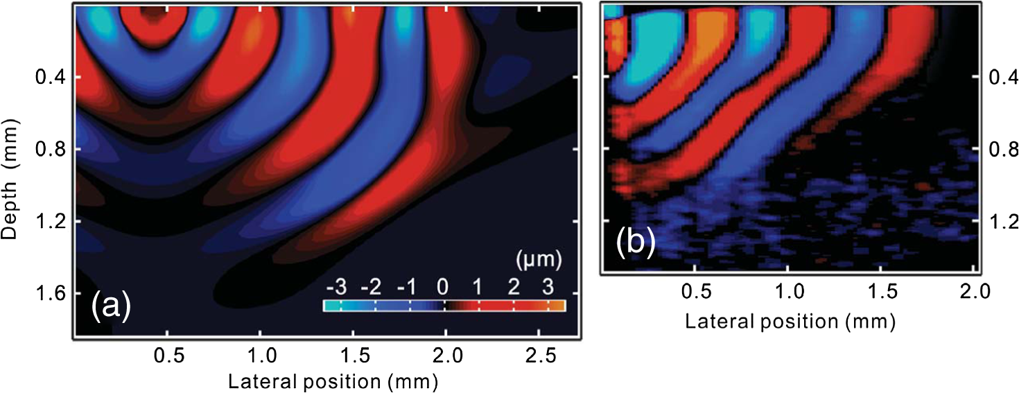

The result of simulation demonstrates the coexisting shear wave and surface wave (Rayleigh wave) modes. Rayleigh wave propagates on the free surface of media, with an active depth of about one wavelength. There is no strict division boundary between the bulk shear wave and Rayleigh wave. The wave field snapshot (Fig. 9) indicates the shear waves with a wavelength of $\sim 0.5 mm$ and Rayleigh wave with a similar velocity. The displacement amplitudes are in good agreement with that from prior literature about the amplidude map of shear waves generated by surface point source.³⁸

4.3.

Shear Waves in Homogenous Phantom

As the wave pattern (spatial-temporal displacement field) is critical for the reconstruction of wave velocity map, the elimination of motion artifact has always been an important issue for all wave imaging modalities. Here, we use a homogeous phantom that is large enough to avoid reflected waves to show the pure shear wave images. As shown in Fig. 6(b), the stimulation source is attached to phantom surface. Figures 10(a1) to 10(a4) show snapshots at four different time instants when the wave propagates within the phantom. The stripe artifacts are clearly noticeable in all the frames. Also, in comparison with the theoretical wavepattern in Fig. 9, the wavefronts exhibit obvious distortion. Figures 10(b1) to 10(b4) show the wave field frames with surface phase compensation. The stripe artifacts and wave distortion are effectively suppressed. The compensated wave pattern still shows a small difference when compared to Fig. 9. This is because the excitations are launched with an angle in the experiments, and also the attenuation is not modeled in the theoretical model. However, the phase images are much more realistic than the artifact-contaminated ones.

Fig. 10

(a1) to (a4) Wave propagating pattern detected with PhS-OCT in a homogenous tissue phantom. (b1) to (b4) Wave pattern after phase compensation. (c1) to (c4) Wave pattern in homogeneous phantom with a layer of oil above. Shown are the snapshots at the time instants of 5, 10, 15, and 20 Ts, where $Ts = sampling period$ . Same colorbar as shown in (a1) applies to each subfigure.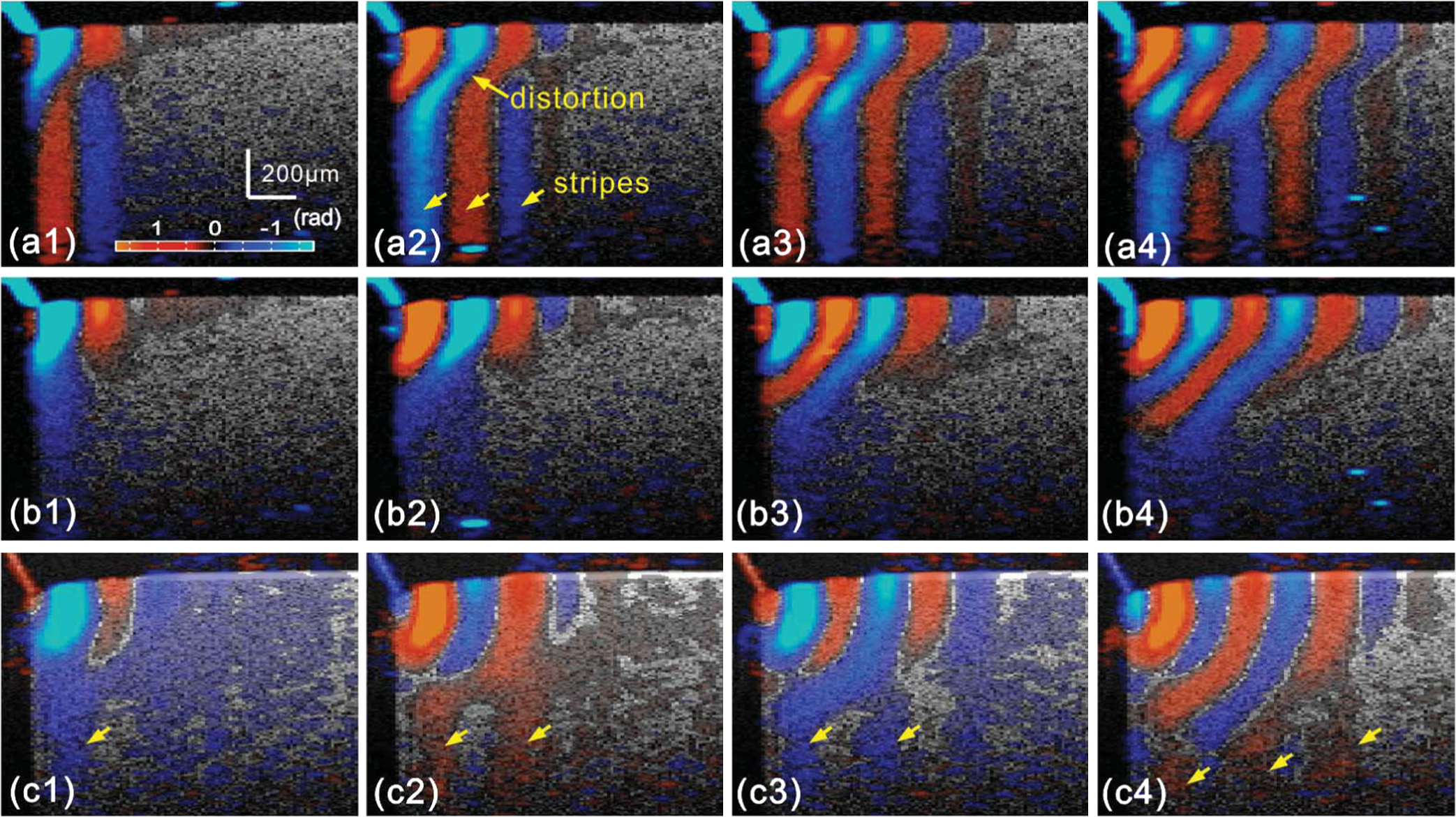

There is a circumstance where the artifacts can be mitigated without compensation. This is shown in Fig. 6(c) where the phantom is placed in a container. We then poured a layer of mineral oil on the surface. To avoid the oil surface motion, we covered the oil layer with a thin glass plate. In this case, the oil layer works as an optical coupling media because the oil has a refractive index that is close to that of phantom, and there is no surface motion on the oil due to the glass plate. The measured wave patterens in this oil-covered phantom are presented in Figs. 10(c1) to 10(c4). It can be seen that the images (without compensation applied) are basically artifact-free. However, as the mineral oil still exhibits a slightly higher refractive index than the phantom ( $\sim 1.42$ versus $\sim 1.33$ ), there exists an opposite stripe, i.e., a very weak amplitude stripe artifact with same phase direction could be observed [as indicated with arrows in Figs. 10(c1) to 10(c4)]. This also confirmed the validity of the compensation method, because for this oil–phantom interface, ( $n_{2} - n_{1}$ ) is a negative value, opposite to the case of air–tissue interface.

5. Conclusions

In this study, the phase-resolved motion detection methods in OCT are briefly reviewed, upon which the formation and characteristics of surface ripple artifact are theoretically and experimentally proved. Furthermore, a method of compensating for these artifacts is proposed accordingly. The artifacts are first observed on a phantom with a moving part and a static part, and then on a homogenous phantom with propagating shear waves and surface waves. For both the cases, the compensation method showed the ability to remove the stripe artifacts and correct the distorted waveforms. As the described circumstances are common in dynamic OCE methods, the compensation algorithm is expected to have wide applications. This investigation also suggests that special attention should be given to the phase errors whenever nonhomogeneous optical medium exists, as the varying refraction expresses a lens effect for phase.

In this work, the refractive index is considered constant and uniform in the specimen. Although a complex sample with large variation of refractive index would complicate the proposed compensation method, it is still reasonable to conclude that, using a rough estimation of refractive index, most of the artifact errors could be eliminated, providing much a higher SNR than leaving this artifact uncorrected. Because the artifact amplitude is ( $n - 1$ ) times the surface displacement, the variation of refractive index has a small variation range in the same type of biological tissue.

One difficulty for this compensation technique is in the situation where the sample surface is uneven or rough. In this case, the optical path would become more complex, leading to complications for interpreting the results. As there already exist very effective algorithms to inversely compute the OCT beam path for refraction correction,³⁹ it is feasible to use this compensation method based on the beam path corrections. However, it is more computation-intensive. Nevertheless, the method given above is only one possible approach for the artifact correction; more effective and robust approaches remain to be explored.

It is hoped that the theoretical analysis and methods reported here will help improve the accuracy of OCT motion detection techniques and advance the developments of a wide range of related biomedical applications.

References

1.

D. Huanget al., “Optical coherence tomography,” Science, 254 (5035), 1178 –1181 (1991). http://dx.doi.org/10.1126/science.1957169 SCIEAS 0036-8075 Google Scholar

2.

P. H. TomlinsR. K. Wang, “Theory, developments and applications of optical coherence tomography,” J. Phys. D Appl. Phys., 38 (15), 2519 (2005). http://dx.doi.org/10.1088/0022-3727/38/15/002 JPAPBE 0022-3727 Google Scholar

3.

W. DrexlerJ. G. Fujimoto, Optical Coherence Tomography: Technology and Applications, Springer-Verlag Berlin(2008). Google Scholar

4.

J. M. Schmitt, “OCT elastography: imaging microscopic deformation and strain of tissue,” Opt. Express, 3 (6), 199 –211 (1998). http://dx.doi.org/10.1364/OE.3.000199 OPEXFF 1094-4087 Google Scholar

5.

J. Rogowskaet al., “Quantitative optical coherence tomographic elastography: method for assessing arterial mechanical properties,” Br. J. Radiol., 79 (945), 707 –711 (2006). http://dx.doi.org/10.1259/bjr/22522280 BJRAAP 0007-1285 Google Scholar

6.

J. Rogowskaet al., “Optical coherence tomographic elastography technique for measuring deformation and strain of atherosclerotic tissues,” Heart, 90 (5), 556 –562 (2004). http://dx.doi.org/10.1136/hrt.2003.016956 1355-6037 Google Scholar

7.

S. J. KirkpatrickR. K. WangD. D. Duncan, “OCT-based elastography for large and small deformations,” Opt. Express, 14 (24), 11585 –11597 (2006). http://dx.doi.org/10.1364/OE.14.011585 OPEXFF 1094-4087 Google Scholar

8.

X. Lianget al., “Optical micro-scale mapping of dynamic biomechanical tissue properties,” Opt. Express, 16 (15), 11052 –11065 (2008). http://dx.doi.org/10.1364/OE.16.011052 OPEXFF 1094-4087 Google Scholar

9.

R. K. WangS. KirkpatrickM. Hinds, “Phase-sensitive optical coherence elastography for mapping tissue microstrains in real time,” Appl. Phys. Lett., 90 (16), 164105 (2007). http://dx.doi.org/10.1063/1.2724920 APPLAB 0003-6951 Google Scholar

10.

R. K. K. WangZ. H. MaS. J. Kirkpatrick, “Tissue Doppler optical coherence elastography for real time strain rate and strain mapping of soft tissue,” Appl. Phys. Lett., 89 (14), 144103 (2006). http://dx.doi.org/10.1063/1.2357854 APPLAB 0003-6951 Google Scholar

11.

R. K. WangA. L. Nuttall, “Phase-sensitive optical coherence tomography imaging of the tissue motion within the organ of Corti at a subnanometer scale: a preliminary study,” J. Biomed. Opt., 15 (5), 056005 (2010). http://dx.doi.org/10.1117/1.3486543 JBOPFO 1083-3668 Google Scholar

12.

S. G. Adieet al., “Audio frequency in vivo optical coherence elastography,” Phys. Med. Biol., 54 (10), 3129 (2009). http://dx.doi.org/10.1088/0031-9155/54/10/011 PHMBA7 0031-9155 Google Scholar

13.

X. Lianget al., “Acoustomotive optical coherence elastography for measuring material mechanical properties,” Opt. Lett., 34 (19), 2894 –2896 (2009). http://dx.doi.org/10.1364/OL.34.002894 OPLEDP 0146-9592 Google Scholar

14.

K. R. Nightingaleet al., “On the feasibility of remote palpation using acoustic radiation force,” J. Acoust. Soc. Am., 110 (1), 625 (2001). http://dx.doi.org/10.1121/1.1378344 JASMAN 0001-4966 Google Scholar

15.

B. F. Kennedyet al., “In vivo three-dimensional optical coherence elastography,” Opt. Express, 19 (7), 6623 –6634 (2011). http://dx.doi.org/10.1364/OE.19.006623 OPEXFF 1094-4087 Google Scholar

16.

C. Liet al., “Determining elastic properties of skin by measuring surface waves from an impulse mechanical stimulus using phase-sensitive optical coherence tomography,” J. R. Soc. Interface, 9 (70), 831 –841 (2012). http://dx.doi.org/10.1098/rsif.2011.0583 1742-5689 Google Scholar

17.

C. Liet al., “Noncontact all-optical measurement of corneal elasticity,” Opt. Lett., 37 (10), 1625 –1627 (2012). http://dx.doi.org/10.1364/OL.37.001625 OPLEDP 0146-9592 Google Scholar

18.

R. Manapuramet al., “Estimation of shear wave velocity in gelatin phantoms utilizing PhS-SSOCT,” Laser Phys., 22 (9), 1439 –1444 (2012). http://dx.doi.org/10.1134/S1054660X12090101 LAPHEJ 1054-660X Google Scholar

19.

M. Razaniet al., “Feasibility of optical coherence elastography measurements of shear wave propagation in homogeneous tissue equivalent phantoms,” Biomed. Opt. Express, 3 (5), 972 –980 (2012). http://dx.doi.org/10.1364/BOE.3.000972 BOEICL 2156-7085 Google Scholar

20.

Y. WangC. LiR. K. Wang, “Noncontact photoacoustic imaging achieved by using a low-coherence interferometer as the acoustic detector,” Opt. Lett., 36 (20), 3975 –3977 (2011). http://dx.doi.org/10.1364/OL.36.003975 OPLEDP 0146-9592 Google Scholar

21.

Y. Zhaoet al., “Real-time phase-resolved functional optical coherence tomography by use of optical Hilbert transformation,” Opt. Lett., 27 (2), 98 –100 (2002). http://dx.doi.org/10.1364/OL.27.000098 OPLEDP 0146-9592 Google Scholar

22.

R. K. WangZ. Ma, “Real-time flow imaging by removing texture pattern artifacts in spectral-domain optical Doppler tomography,” Opt. Lett., 31 (20), 3001 –3003 (2006). http://dx.doi.org/10.1364/OL.31.003001 OPLEDP 0146-9592 Google Scholar

23.

G. HaM. W. Lindner, “‘Coherence radar’ and ‘spectral radar’—new tools for dermatological diagnosis,” J. Biomed. Opt., 3 (1), 21 –31 (1998). http://dx.doi.org/10.1117/1.429899 JBOPFO 1083-3668 Google Scholar

24.

L. Anet al., “High speed spectral domain optical coherence tomography for retinal imaging at 500,000 A-lines per second,” Biomed. Opt. Express, 2 (10), 2770 (2011). http://dx.doi.org/10.1364/BOE.2.002770 BOEICL 2156-7085 Google Scholar

25.

S. ChinnE. SwansonJ. Fujimoto, “Optical coherence tomography using a frequency-tunable optical source,” Opt. Lett., 22 (5), 340 –342 (1997). http://dx.doi.org/10.1364/OL.22.000340 OPLEDP 0146-9592 Google Scholar

26.

B. Potsaidet al., “Ultrahigh speed 1050 nm swept source/Fourier domain OCT retinal and anterior segment imaging at 100,000 to 400,000 axial scans per second,” Opt. Express, 18 (19), 20029 (2010). http://dx.doi.org/10.1364/OE.18.020029 OPEXFF 1094-4087 Google Scholar

27.

M. A. Chomaet al., “Sensitivity advantage of swept source and Fourier domain optical coherence tomography,” Opt. Express, 11 (18), 2183 –2189 (2003). http://dx.doi.org/10.1364/OE.11.002183 OPEXFF 1094-4087 Google Scholar

28.

Y. Zhaoet al., “Real-time phase-resolved functional optical coherence tomography by use of optical Hilbert transformation,” Opt. Lett., 27 (2), 98 –100 (2002). http://dx.doi.org/10.1364/OL.27.000098 OPLEDP 0146-9592 Google Scholar

29.

R. E. Setchell, “Refractive index of sapphire at 532 nm under shock compression and release,” J. Appl. Phys., 91 (5), 2833 –2841 (2002). http://dx.doi.org/10.1063/1.1446219 JAPIAU 0021-8979 Google Scholar

30.

T. RoystonH. MansyR. Sandler, “Excitation and propagation of surface waves on a viscoelastic half-space with application to medical diagnosis,” J. Acoust. Soc. Am., 106 (6), 3678 (1999). http://dx.doi.org/10.1121/1.428219 JASMAN 0001-4966 Google Scholar

31.

E. A. ZabolotskayaY. A. IlinskiiM. F. Hamilton, “Nonlinear surface waves in soft, weakly compressible elastic media,” J. Acoust. Soc. Am., 121 (4), 1873 (2007). http://dx.doi.org/10.1121/1.2697098 JASMAN 0001-4966 Google Scholar

32.

C. Liet al., “Evaluating elastic properties of heterogeneous soft tissue by surface acoustic waves detected by phase-sensitive optical coherence tomography,” J. Biomed. Opt., 17 (5), 057002 (2012). http://dx.doi.org/10.1117/1.JBO.17.5.057002 JBOPFO 1083-3668 Google Scholar

33.

U. Hamhaberet al., “Comparison of quantitative shear wave MR-elastography with mechanical compression tests,” Magn. Reson. Med., 49 (1), 71 –77 (2003). http://dx.doi.org/10.1002/(ISSN)1522-2594 MRMEEN 0740-3194 Google Scholar

34.

R. K. WangZ. Ma, “A practical approach to eliminate autocorrelation artefacts for volume-rate spectral domain optical coherence tomography,” Phys. Med. Biol., 51 (12), 3231 (2006). http://dx.doi.org/10.1088/0031-9155/51/12/015 PHMBA7 0031-9155 Google Scholar

35.

A. R. Levander, “Fourth-order finite-difference P-SV seismograms,” Geophysics, 53 (11), 1425 –1436 (1988). http://dx.doi.org/10.1190/1.1442422 GPYSA7 0016-8033 Google Scholar

36.

I. M. HallajR. O. Cleveland, “FDTD simulation of finite-amplitude pressure and temperature fields for biomedical ultrasound,” J. Acoust. Soc. Am., 105 (5), L7 (1999). http://dx.doi.org/10.1121/1.426776 JASMAN 0001-4966 Google Scholar

37.

J. Virieux, “P-SV wave propagation in heterogeneous media: velocity-stress finite-difference method,” Geophysics, 51 (4), 889 –901 (1986). http://dx.doi.org/10.1190/1.1442147 GPYSA7 0016-8033 Google Scholar

38.

S. Cathelineet al., “Diffraction field of a low frequency vibrator in soft tissues using transient elastography,” IEEE Trans. Ultrason. Ferroelectr. Freq. Control, 46 (4), 1013 –1019 (1999). http://dx.doi.org/10.1109/58.775668 ITUCER 0885-3010 Google Scholar

39.

S. Ortizet al., “Optical distortion correction in optical coherence tomography for quantitative ocular anterior segment by three-dimensional imaging,” Opt. Express, 18 (3), 2782 –2796 (2010). http://dx.doi.org/10.1364/OE.18.002782 OPEXFF 1094-4087 Google Scholar

Citation Download Citation

Shaozhen Song, Zhihong Huang, and Ruikang K. Wang "Tracking mechanical wave propagation within tissue using phase-sensitive optical coherence tomography: motion artifact and its compensation," Journal of Biomedical Optics 18(12), 121505 (22 October 2013). https://doi.org/10.1117/1.JBO.18.12.121505

Published: 22 October 2013

Access the abstract

JOURNAL ARTICLE
10 PAGES

DOWNLOAD PAPER SAVE TO MY LIBRARY

GET CITATION

CITATIONS

Cited by 108 scholarly publications and 2 patents.

Explore citations on Lens.org

RIGHTS & PERMISSIONS

Get copyright permission Get copyright permission on Copyright Marketplace

KEYWORDS

Wave propagation

Optical coherence tomography

Tissues

Natural surfaces

Tissue optics

Refractive index

Fused deposition modeling

1.

Introduction

2.

Theoretical Aspects

2.1.

Phase-Resolved OCT Motion Detection

Fig. 1

Eq. (1)

Eq. (2)

Eq. (3)

Eq. (4)

2.2.

Artifacts Induced by Air Interface Motion

Fig. 2

Eq. (5)

Eq. (6)

Eq. (7)

Eq. (8)

Eq. (9)

Eq. (10)

3.

Methods

3.1.

Experimental Setup

Fig. 3

3.2.

Phantom Preparation

3.3.

Scan Protocol and Reconstruction of Displacement Field

Fig. 4

3.4.

Modeling of Surface and Shear Wave Pattern

Fig. 5

Eq. (11)

Eq. (12)

4.

Results

4.1.

Presence of Artifact

Fig. 6

Fig. 7

Fig. 8

4.2.

Wave Field Simulation

Fig. 9

4.3.

Shear Waves in Homogenous Phantom

Fig. 10

5.

Conclusions

References

Show All Keywords

Keywords/Phrases

Search In:

Publication Years