Fast, broadband, rugged spectrometer for near-infrared measurements of organic solutions and multicomponent mixtures

Ricardo Claps; Jeffrey Virojanapa

doi:10.1117/1.JBO.18.11.117001

1 November 2013 Fast, broadband, rugged spectrometer for near-infrared measurements of organic solutions and multicomponent mixtures

Ricardo Claps, Jeffrey Virojanapa

Author Affiliations +

Journal of Biomedical Optics, Vol. 18, Issue 11, 117001 (November 2013). https://doi.org/10.1117/1.JBO.18.11.117001

Abstract

The mode of operation and theoretical concept behind a type of near-infrared spectrometer is discussed, which is used to measure concentrations of glucose, ethanol, CaCl ₂ , and KCl solutions in water, respectively. The main features of the instrument are its potential for short time-to-measurement resolution on the order of tens of milliseconds, its broad spectral bandwidth from 1.0 to 2.4 μm, and its ruggedness. These features allow the device to operate remotely in field applications and to utilize a wide variety of optical interfaces based on state-of-the-art fiber optic technology. Also, they provide a straightforward path to miniaturization with the concomitant enhancement in time resolution and applicability of the instrument and the technique.

1. Introduction

Current trends in spectroscopy are oriented toward the development of instrumentation that can be used outside the laboratory in applications such as in a surgery room, a primary-care clinic, or even a primary-care physician’s office.¹ This framework imposes severe conditions on the performance of spectroscopic systems in terms of ruggedness, simplicity, and speed of operation. At the same time, device sensitivity and specificity is expected to be comparable with laboratory-grade instrumentation. Added to this is the need to assess a multiplicity of components for every sample, either because each of these components is important for a given clinical configuration or because some of these components may interfere in the correct assessment of the signal as spurious background and need to be subtracted out.

This article presents the concept and realization of an instrument that is designed to satisfy the above requirements. The development of the instrument comprises a computational algorithm and a hardware associated with it. The algorithm component of the instrument is a discretized version of multivariate linear regression (dMLR). The hardware component is based on a rotary optical switch developed and patented by Neptec Optical Solutions, Inc. (NOS, Fremont, California) and referred to as RadiaLight® switch.² Both dMLR and RadiaLight® are intimately related, but the dMLR algorithm has a broader range of applicability, whereas the hardware may adopt different configurations in future developments.

2. Discrete Multivariate Linear Regression Analysis

In the most general mode, a set of $n$ measurements performed on $m$ different samples can be organized in the form of an $n \times m$ matrix, $P$ . In MLR, the matrix, $P$ , is factorized in the form:³

Eq. (1)

P = R \cdot C .

In Eq. (1), $R$ is an $n \times r$ matrix, representing the calibration of the system with known values of the experimental setup, and $C$ is an $r \times m$ matrix, representing the unknown composition of the principal components in the sample being measured. The elements of matrix $C$ are the actual properties of the sample that need to be measured. For practical reasons, matrix $C$ will be referred to as the “concentrations” matrix. The $r$ columns of matrix $R$ are called “loading vectors” and correspond to the invariant properties of the measurement platform. Equation (1) establishes that a linear relationship exists between the “concentrations” in the experiment, $C$ , and the measurement results, $P$ . This is a fundamental hypothesis of MLR, and its validity needs to be verified in each case where it is applied. This will be hereafter referred to as the “linear hypothesis.” Once matrix $R$ is determined, then solving Eq. (1) for $C$ is straightforward, as in:

Eq. (2)

C = {(R^{T} \cdot R)}^{- 1} \cdot R^{T} \cdot P .

In Eq. (2), it is assumed that the matrix, $ξ \equiv (R^{T} \cdot R)$ , is nonsingular (otherwise, matrix $R$ is ill-defined, and the measurement strategy needs revision). Note that the procedure described by Eqs. (1) and (2) is quite general and involves a measurement that can be as detailed as desired, since the dimensions of matrices $P$ and $C$ are arbitrary. Matrix $R$ is formed by previous knowledge of the experimental conditions in which the measurement will be carried out. This procedure uses a given number of sampling measurements or calibrations with known concentrations, $\tilde{C}$ . An example is the measurement of glucose concentrations in aqueous solutions using near-infrared (NIR) spectroscopy. A calibration procedure starts by measuring a control set of glucose solutions in water, e.g., 70 different samples with monotonically increasing, known glucose concentrations, and everything else remains the same in the experiment. Labeling the calibration concentrations and calibration measurements as $\tilde{C}$ and $\tilde{P}$ , respectively, we can find the matrix $R$ from Eq. (1), as

Eq. (3)

R = \tilde{P} \cdot {\tilde{C}}^{t} {(\tilde{C} \cdot {\tilde{C}}^{t})}^{- 1} .

Figure 1 shows the NIR spectra of glucose and water solutions with varying glucose concentrations from $10 mg / dL$ up to $35 g / dL$ . The spectra were collected using a grating-based spectrometer having a 6-nm spectral resolution (Ocean Optics, Inc., Dunedin, Florida) with a 256-pixel InGaAs photodetector array. The resolving power of the instrument is thus approximately 250. The Ocean Optics spectrometer requires the collection of the spectrum in two patches to correct for second-order diffraction effects from the grating: the spectrum from 1750 to 2500 nm is collected using a long-pass filter with transmission edge at 1700 nm. The samples were placed in a glass cuvette with a 2-mm optical path, and the optical source is a broadband emission lamp emitting a total of 7 W of power (HL2000 Ocean Optics, Inc.) with a UV-visible filter to prevent the water from heating during the measurements.

Fig. 1

Near-infrared (NIR) spectra of aqueous solutions of glucose with varying concentration: from 10 up to $500 mg / dL$ in increments of $10 mg / dL$ ; thereafter, in increments of $500 mg / dL$ up to $10 g / dL$ ; and thereafter in increments of $5 g / dL$ up to $35 g / dL$ . Each spectrum is centered about its mean and has been corrected for temperature fluctuations.

The ordinate in Fig. 1 represents a normalized differential spectrometer signal using distilled water as a baseline. To obtain the baseline, a spectrum of distilled water was collected at a reference temperature. For every glucose solution measurement, the temperature of the solution was measured using a thermocouple. The reference water spectrum (“ $w$ ”) was “corrected” for temperature (see Appendix B), and then it was subtracted from the glucose solution spectrum (“ $g$ ”) to yield a differential spectrum (“ $g - w$ ”). Temperature correction of the glucose solution spectrum consists of transforming the reference water spectrum from a reference temperature to the glucose measurement temperature. The result is normalized to the sum of the glucose and the water spectra (“ $g + w$ ”). Thus, the ordinate “ $y$ ” in Fig. 1 is $y = (g - w) / (g + w)$ .

Temperature is one of the factors that strongly affects NIR water spectra even for $T$ fluctuations of about 0.1°C. Thus, temperature needs to be taken into account for any measurement involving aqueous solutions.⁴ One way of doing this is by collecting the calibration spectra using a thermal bath, ensuring a $T$ fluctuation of less than 0.1°C (in the case of aqueous solutions of glucose⁵). The procedure followed in the present work uses the previous recording of the spectra of pure water as a function of temperature to build a calibration chart that can be compared against each sample spectra. This requires measuring temperature for every spectrum collected. Details about the procedure will be discussed in Appendix B.

3. Discretization

Mathematically, the process of discretization can be viewed simply as a weighted summation of matrix components over a certain number, $d$ , of elements. This is described in Eq. (4) below:

Eq. (4)

{\tilde{R}}_{i k} = \sum_{j}^{d - 1} β_{i} \cdot R_{(i \cdot d + j) k} .

The factor $β_{i}$ is a weighting parameter to be adjusted in the process of optimization, also defined herein as training or calibration of the instrument in question. This optimization procedure is based on a given measure of performance for the system, e.g., minimization of the measurement error for glucose concentrations, as described in detail in Appendix A. The dimensionality of the MLR problem is then reduced from $n$ to $n^{'} = n / d$ , reducing the computational time and the hardware requirements concomitantly. However, an operation such as the one described in Eq. (4) carries the cost of information loss due to reduced precision. On the other hand, discretization reduces data “graininess,” increasing information content of the reduced dataset. The balance between these competing effects can be quantified in different ways: one useful procedure is through the use of the relative entropy matrix (REM).⁶ In REM, a variable is defined that quantifies the information content of a given dataset. This is called the “entropy of the pooled dataset.” In the case of MLR analysis, the pooled dataset is matrix $C$ , which contains information of the instrument calibration. The entropy is defined as

Eq. (5)

E_{n} (k) = - \frac{1}{\ln n} \sum_{j = 1}^{n} R_{j k} \ln (R_{j k}) .

By maximizing the entropy, $E_{n}$ , the dataset is guaranteed to carry the maximum possible information content.⁷ Equation (5) actually refers to a “relative” entropy measure, assuming a maximum normalized value of $E_{n} (k) = 1$ . The parameter $k$ is a counting index given by $1 \leq k \leq m$ , and $m$ is the total number of different records of data available, which in the case of matrix $R$ would be the total number of loading vectors to be used. A variance in the average relative entropy, or entropy variance, is then defined as

Eq. (6)

δ R {(n)}^{2} = \frac{1}{M - 1} \cdot \sum_{k = 1}^{m} {(E_{n} (k) - {〈 E_{n} (k) 〉}_{n})}^{2} .

Since entropy becomes indeterminate for extreme values of the data size, $n$ , such as $n = 1$ or $n$ approaching infinity, a more convenient criterion to characterize the information content of a given dataset is the minimization of the entropy variance, $δ R (n)$ [Eq. (6)].

Figure 2 shows the result of applying the concept in Eqs. (5) and (6) to the problem of using NIR spectroscopy for measuring glucose concentration in aqueous solutions. In this case, the variable $M$ [Eq. (6)] expresses the aqueous solutions with different concentrations of glucose. The goal is to find the number of measurement channels, $n$ , that maximizes the information content, while keeping device cost and complexity at a minimum. The spectra used in the calculations are shown in Fig. 1. The data consists of arrays, $R_{k}$ , with 256 data points, each point representing the signal level on a specific pixel of the InGaAs photodetector array for a given wavelength dispersed by a diffraction grating. The data points can be “binned” together (averaged) in sets of different sizes, resulting in a varying number of channels or (bins) into which the data is distributed. As the binned array size is reduced (thus, increasing the number of channels), according to Eq. (4), the variance in the entropy shows a pattern analogous to that of the well-known Allan variance plots.⁸ Based on this analysis, the conclusion is that to determine glucose concentration in an aqueous solution by using NIR spectra in the 850 to 2500-nm wavelength range, the ideal number of data binning (i.e., the number of measurement channels required in the instrument) should be somewhere between 10 and 20. Other authors have used the ideas of information entropy and MLR in order to optimize the sensitivity and specificity of a spectroscopic system,⁹ but not within the framework of the data discretization algorithm proposed here.

Fig. 2

Entropy variance as a function of the array size for “ $m$ ” sets of NIR spectra of glucose solutions ( $m = 71$ ). The optimal array size, $n$ , is between 10 and 20 channels or bins.

The calculations used to obtain an optimized set of filters involve the use of a stochastic scan of the 24-dimensional parameter space that spans all possible sets of eight interference filters, each with a given center wavelength, bandwidth, and weight factor ( $λ_{c}$ , $Δ λ_{c}$ , and $κ$ , respectively). Note that the weight factor, $κ$ , can be any real number, positive or negative, and it is applied to the integrated signal coming from any given filter. This weight factor, $κ$ , is analogous to the factor, $β_{i}$ , in Eq. (4), except that the latter implies the validity of the linearization hypothesis. Using a statistically significant set of sample spectra with glucose concentrations ranging from 10 up to $500 mg / dL$ (a subset of the spectra shown in Fig. 1), the optimization routine selects the filter set that minimizes the relative variance in the data. The result of the optimization routine is shown in Figs. 3 and 4, where a linear correlation is found between a suitable variable, $S$ , and the glucose concentration of the solution, [ $g$ ]. The variable, $S$ , is a combination of operations performed on the “discretized,” eight-dimensional signal produced by the electromagnetic radiation detected through the eight interference filters using a single photodetector. This will be discussed in detail in the next section.

Fig. 3

Eight interference filters selected for glucose/water discrimination. The routine can be implemented assuming different profiles for the filters; the case illustrated is a flattened Gaussian. The continuous, gray curve shows the features of the glucose/water difference spectra that the optimization routine uses to maximize the discrimination (glucose concentration, $[g] = 35 g / dL$ ). The left vertical axis shows a weighting factor, $κ$ , and the right shows a spectral weight for the glucose/water mixture.

Fig. 4

Result of the discretized version of multivariate linear regression (dMLR) optimization procedure in terms of a linear correlation between the parameter $S$ and the glucose concentration of the samples. The resulting linear fit is shown in the figure. The modeled instrument uses eight signal channels with their corresponding interference filters, as shown in Fig. 3.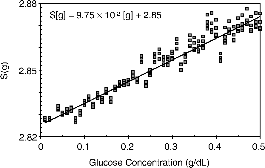

Figure 5 shows a histogram of the error between the calculated and the actual concentrations of glucose in the samples used. The calculated glucose concentrations are obtained using the eight interference filters illustrated in Fig. 3. The standard deviation from the straight line in Fig. 4 shows that more than 80% of the data points lay within an error of $50 mg / dL$ in concentration measurement. The average error in the measurement is $25 mg / dL$ for aqueous solutions of glucose with concentration ranging from 10 to $500 mg / dL$ . These results are within clinical validity for the diagnosis and treatment of diabetes and compare satisfactorily with state-of-the-art optical instrumentation for this purpose.¹⁰^–²² More importantly, the significance of this result is that a dMLR-based instrument would be able to perform the measurement within a 10-s time resolution, and even less time if simple improvements in the hardware are introduced. Details of the hardware and instrumentation will be described in the next section. The stochastic parameter scan routine used to optimize the performance of the discretized channel set will be described in Appendix A.

Fig. 5

Histogram of the error in the data samples shown in Fig. 4 ( $mg / dL$ ). The aggregated plot at the bottom shows that in the ideal case, this instrument would produce an error of less than $50 mg / dL$ in more than 75% of the samples.

4. Spectrometer

The architecture of the device is depicted in Fig. 6. The concept is analogous to a previous work by NOS, where the goal was to measure cholesterol, collagen, and elastin concentrations for cardiovascular angiography applications.²³ The instrument makes use of interference filters and homogeneous integration of the signal across the filter pass-band with a single photodetector. In the actual experiments, a total of nine interference filters were selected to maximize the measurement accuracy for an aqueous glucose solution.

Fig. 6

Glucose sensor architecture. The lamp provides broadband electromagnetic radiation that is passed through a number of filters, $f_{i}$ , in each channel of the rotary switch (RadiaLight®). The output from the rotary switch is split between the glucose sample solution (detector A) and a pure water reference signal (detector B). The signal is processed by subtracting the measurements in detector B to that in detector A for each filter and normalizing the measurement to the sum of the two signals.

To place the glucose measurement technique within the framework of dMLR, as detailed in Eqs. (1)–(3), it is useful to define a new variable, $S$ , as in Eq. (7):

Eq. (7)

S = \sqrt{\sum_{i} {[1 - κ_{i} \cdot (A_{i} - B_{i}) / (A_{i} + B_{i})]}^{2}} .

In Eq. (7), $A_{i}$ is the signal in filter “ $i$ ” (denoted $f_{i}$ , cf. Fig. 6) related to the sample (e.g., a given concentration of glucose in pure water solution), and $B_{i}$ is the signal in $f_{i}$ related to a reference sample (e.g., pure water). The glucose concentration, [ $g$ ], is obtained from $S$ by a linear expression,

Eq. (8)

[g] = K_{g} \cdot S + b .

In Eq. (8), $K_{g}$ and $b$ are regression coefficients. Equations (7) and (8) express [ $g$ ] as a nonlinear function of the signal measured from the sample, ${\vec{A}}^{t} = (A_{1}, A_{2}, \dots, A_{n})$ . This clearly contradicts the basic assumption of MLR, as stated in Eq. (1). It is well known, however, that under low-glucose concentration conditions, $\vec{A} \approx \vec{B}$ , Eq. (7) can be approximated as

Eq. (9)

S \approx \sqrt{n} \cdot (1 + \frac{{\vec{B}}^{T} \cdot \vec{v}}{2} - \frac{{\vec{A}}^{T} \cdot \vec{v}}{2}) .

In Eq. (9), the vector, $\vec{v}$ , is given by

Eq. (10)

{\vec{v}}^{t} = (κ_{1} / B_{1}, κ_{2} / B_{2}, \dots, κ_{n} / B_{n}) .

Making the following associations,

Eq. (11)

b = - K_{g} \cdot \sqrt{n},

Eq. (12)

{(R^{T} \cdot R)}^{- 1} \cdot R^{T} = \frac{K_{g}}{2} [{\vec{v}}^{t}]

Eq. (13)

P = [\vec{B} - \vec{A}]

Eq. (14)

C = [g],

it turns out that Eq. (8) can be written for

C = [g]

as

Eq. (15)

C = {(R^{T} \cdot R)}^{- 1} \cdot R^{T} \cdot P .

Matrix $R$ in this case is a matrix having only one dimension corresponding to the principal component in the problem at hand (the glucose concentration). In other words, $R$ in the present problem is a vector that can be extracted from Eq. (12) as

Eq. (16)

R = (\frac{2}{K_{g}}) \cdot {(\vec{v} \cdot {\vec{v}}^{t})}^{- 1} \cdot [\vec{v}] .

In essence, the dMLR procedure here consists of finding the values of ( $f_{i}$ , $δ f_{i}$ , $κ_{i}$ ) such that the linearity in Eq. (8) is satisfied and such that the error (variance) in the measurement, $σ_{\max}$ , is minimized. This is equivalent to finding suitable values of $β_{i}$ in Eq. (4).

5. Experiment and Results

Figure 7 shows the spectral profiles of the nine interference filters used in the instrument described in Fig. 6. The filter set covers a wavelength range in the NIR domain from 0.9 to 2.3 μm. Note that the band-pass filters used in the instrument do not match exactly the band-pass filters specified by the stochastic method (shown in Fig. 3) and used in the theoretical calculations that generated Figs. 4 and 5. The reason for this is the stronger photodetector signal provided by broader pass-band filters, at the cost of reducing specificity in the measurement. The results of the experiments performed using an instrument with the architecture shown in Fig. 6 and the filters from Fig. 7 are illustrated in Figs. 8 Fig. 9–10. Figure 8 shows the time trace of the signal measured through each of the nine channels. The device operated at 300 RPM, and data were averaged 50 times, leading to a total time-to-measurement resolution of 7.5 s. The signal-to-noise ratio (SNR) obtained for the detector used is $\sim 10^{3}$ . The SNR is not the same for all the filters used, as can be seen from Fig. 8. The highest SNR is obtained for the filter with broadest bandwidth, namely filter no. 2 centered at 1235 nm (cf. Figs. 7 and 8). Using the current instrument, the speed of the RadiaLight® motor can be increased by a factor of 20 for a time-to-measurement resolution of 375 ms. Further noise-reduction techniques like Kalman filtering²⁴ and auto-balance feedback circuitry²⁵ can be used to completely eliminate the need for averaging the signal. This would bring the achievable time-to-measurement resolution down to less than 10 ms.

Fig. 7

Spectral profile of the nine filters used in the instrument depicted in Fig. 6. The labels on top of each peak indicate their order in the time-domain sequence of the corresponding signal, as shown in the trace for Fig. 11.

Fig. 8

Time sequence of signals from nine channels representing the photodetector output signal as a function of time from five different solutions containing: (1) glucose in water ( $35 g / dL$ ), (2) pure ethanol, (3) cholesterol in water ( $100 mg / dL$ ), (4) KCl in water ( $1 g / dL$ ), and (5) ${CaCl}_{2}$ in water ( $1 g / dL$ ). Signal-to-noise ratio (SNR) is 1000.

The traces in Fig. 8 correspond to five different aqueous solutions, including glucose (at $35 g / dL$ ), all of them relevant for biomedical applications. Figure 9 shows the $S ([g])$ correlation curves obtained for one set of aqueous glucose solutions measured on 4 different days. For each correlation curve, the sample set was measured in a random sequence relative to sample concentration. The linear nature of the data points shown in Fig. 9 for each of the sample set collections proves the validity of principal component analysis when used with the architecture depicted in Fig. 6 for the measurement of glucose in water. The reason for the difference between the correlations shown in Fig. 9 and that obtained theoretically (cf. Fig. 4) is the different filter set used. Notice that, as expected, the broader pass-band of the filters used in the experiment results in a reduced specificity of the correlation, leading to a reduced measurement accuracy of about $1 g / dL$ . The slope of the correlations obtained experimentally (Fig. 9) is about 50 times lower than that shown in Fig. 4. This is a reflection of the lower specificity obtained from using broadband-pass filters, and a result of the nonlinear nature of electromagnetic radiation absorption, considering the fact that Fig. 4 relates to low-glucose concentration levels ( $< 0.5 g / dL$ ), whereas Fig. 9 relates to glucose concentrations 1 to 2 orders of magnitude greater. Each data collection set in Fig. 9 was performed within a day difference from one another. Specifically, the dataset with the highest slope ( $K_{g} = 0.0026$ ) is the earliest data collection set, corresponding to the freshly prepared samples. The next collection set corresponds to the second largest slope ( $K_{g} = 0.0023$ ), one day after the first collection set. The third collection set corresponds to the third largest slope ( $K_{g} = 0.0020$ ), one day after the second; and the fourth collection set corresponds to the lowest slope ( $K_{g} = 0.017$ ), one day after the third. During the four data collection sequences, the sample set was stored in polystyrene cups under refrigeration at about 3°C. The data show sample degradation, which may be due to ambient water condensation in the sample container or glucose diffusion into the polystyrene container walls. The offset value “ $b$ ” [cf. Eq. (8)] does not show a consistent pattern in terms of the time of measurement; thus, it is not possible with the present data to establish the origin of the change in offset values. In practical terms, the day-to-day use of an instrument as presented in Fig. 9 hinges on the linear response across the large dynamic range demonstrated. For routine measurements, two or three reference points may be needed as a calibration to find the linear regression curve. For example, two, three, or more reference samples with known glucose concentrations may be placed in photo-detector A (PD A) port (Fig. 6) for every measurement event. Given the speed of every single measurement (e.g., 10 ms per data point), the addition of the reference sample calibration steps is not deleterious to the overall measurement protocol. The reference samples may be calibrated periodically: once a day, once a week, or less often, according to the conditions of storage and other environmental factors. In a further development, the use of blood samples would be interesting. In this case, a new filter set needs to be determined using detailed spectroscopic analysis similar to what is described in Figs. 1–4.

Fig. 9

Correlation of $S (g)$ to the concentration of glucose in water, where $S$ is as defined in Eq. (8) and where the data used was obtained with an instrument as shown in Fig. 6. Four datasets collected in different days from the same sample set were used.

The use of a filter set that has been optimized for the measurement of glucose in water does not preclude the application of the same filter set for the measurement of other solutions of relevance in biomedical research. Figure 10 shows the performance of the instrument for the measurement of water solutions of ${CaCl}_{2}$ , KCl, and ethanol. The differential solution measurements with a water baseline were temperature-corrected just like the glucose measurements $[g]$ above (also, see Appendix B). The differential measurement scheme using distilled water as a baseline is as depicted in Fig. 6. The linear correlations obtained are quite remarkable, considering the fact that the filter set was optimized for glucose solutions. In particular, it is seen that the ethanol correlation renders a precision of $\sim 2 %$ in concentration measurement. This is an upper bound for the measurement error, since it includes the sample preparation error which cannot be estimated due to the lack of a separate, more precise measurement technique in our lab when this testing was conducted. Other instruments have achieved a better sensitivity,²⁶ but with a highly reduced measurement speed of tens of seconds. In the case of ${CaCl}_{2}$ and KCl, the measurement error, including sample variability, is in the range of clinically relevant electrolyte concentrations in blood.²⁷ For ${CaCl}_{2}$ , for example, 80% of the measurements are within $0.5 g / dL$ of the sample preparation value, and for KCl, 80% of the measurements lie within $0.4 g / dL$ of the sample preparation value. While the present ion-concentration measurements are not taken simultaneously, nor correlated with a corresponding parallel calibration, it is noteworthy that the accuracy for each analyte is better than the other values reported in the literature (e.g., results in Ref. 22). While it might be argued that the results in Ref. 22 were collected from real blood samples, it is also true that the FT-spectrometer used in Ref. 22 has a resolving power of 16,000 in the spectral region from $400$ to 1162 nm and 8000 in the spectral region 833 to 2631 nm. Again, results are hard to compare on a one-to-one basis, but the overall comparison with our device is at least encouraging.

Fig. 10

Linear correlations, $S$ , obtained with the instrument depicted in Fig. 9 for water solutions of (a) ${CaCl}_{2}$ (mean error $0.2 g / dL$ ), (b) KCl (mean error $0.2 g / dL$ ), and (c) ethanol (mean error 2%).

6. Discussion

The first issue to tackle is the validity of the linearity assumption implicit in the analysis used to interpret the data. Equations (7)–(16) demonstrate that the linear approach is valid, at least for situations in which the effect of the analyte in the optical signal is a perturbation relative to the reference signal. This means: $| 1 - ‖ A ‖ / ‖ B ‖ | ≪ 1$ , with $A$ and $B$ as used in Eq. (7). More generally, the use of a broadband signal and a suitably selected channel set guarantees that the linearity of Eq. (1) is kept well beyond the linearity requirement for a single channel in the instrument. Such requirements are set forth by physical models like the Beer–Lambert law of absorption, which are meaningful across narrow wavelength bands. In Appendix B, it will be demonstrated that the ability to select different spectral regions of the signal, across a wide spectral range with suitable weight factors, $β_{i}$ [Eq. (4)], largely increases the linear range of the parameter, $S$ [cf. Eq. (7)]. Suffice to say that, as Fig. 9 demonstrates, the dynamic range for glucose concentration measurements extends for almost 3 orders of magnitude. This result, to the best of the authors’ knowledge, has no precedent in the literature of glucose sensors. While perhaps the detection range for glucose lies well beyond clinically sensitive values, the reader may realize that such a broad dynamic range is not dependent on the analyte. Figure 11 shows loading vectors for the aqueous solutions depicted in Fig. 10 (namely, ${CaCl}_{2}$ , KCl, ethanol, and glucose).

Fig. 11

Measured values of the “loadings” vectors associated with the concentration of glucose (diamonds), calcium chloride (horizontal bars), potassium chloride (squares) and ethanol (triangles), all in water.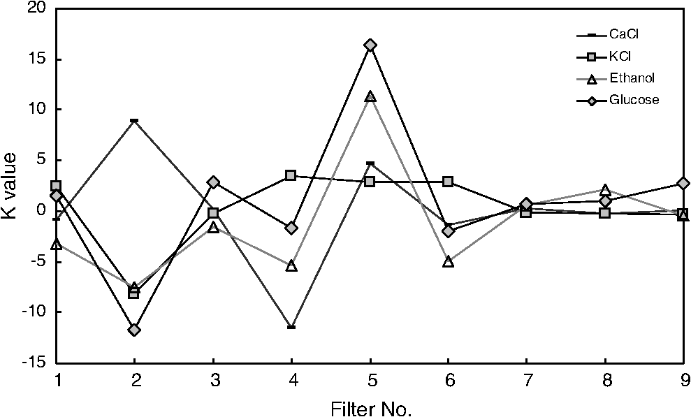

To discuss Fig. 11 in more detail, we will focus on the glucose case. The NIR spectrum of aqueous glucose solutions has been extensively studied in the past decade, concurrently with efforts to develop noninvasive optical methods for the treating and monitoring of diabetes.¹⁰^–²²^,²⁸

The NIR absorption in the overtone band (approximately from 1100 to 1800 nm) consists mostly of water lines (cf. Fig. 1) including a very strong band at $\sim 1450 nm$ and a much weaker glucose band at $\sim 1680 nm$ . In the combination band region (1900 to 2500 nm), there is a very strong water band at $\sim 1990 nm$ and two or three weaker glucose absorption features (1900 to 2300 nm). Notably, the presence of glucose in solution produces a profound effect in the spectral signature of water absorption lines, both in the overtone and in the combination band regions. This effect is associated with line shifting and broadening of the main water lines, together with the “substitution” effect, whereby water absorption is reduced in certain ranges as water molecules are replaced by glucose in the solution. The contribution of refractive effects to the spectra shown is minimal, as demonstrated in Appendix B.

The use of glucose absorption lines in the NIR-combination band range (1.9 to 2.3 μm) for noninvasive diabetes monitoring has been implemented by several authors.⁴^,⁵^,¹⁰^,¹⁹ Prior attempts faced the problem of weak absorption with varying degrees of success. Furthermore, the absorption lines in the NIR range may be overwritten by the strong water absorption band at 1990 nm. Some groups have attempted to overcome this problem by using stronger glucose absorption bands in the mid-IR region (9 to 10 μm).¹⁷^,²⁰ However, the instrumentation for this wavelength range becomes more complex, and scattering issues still permeate the data analysis process. Interestingly, Ref. 17 presents a spectroscopic system having a plurality of 25 discrete filters in the mid-IR spectral domain. The results reported in Ref. 17 are comparable with the model data fit for glucose described above (cf. Fig. 4), while it omits a discussion of how the filters were selected. The analysis presented herein suggests that the authors in Ref. 17 presumably could reduce their filter set by about half. Albeit the spectral ranges between Ref. 17 (mid-IR) and our results (NIR) are different, it is expected that the information content in the mid-IR be higher due to the presence of stronger glucose absorption peaks in this region. Thus, the “knee” of the Allan variance plot shown in Fig. 2 should occur at a lower value of “ $n$ ” for the mid-IR data, relative to the NIR-data.

The instrument presented in this article measures the optical signal across a broad spectral band and is able to include overtone and combination bands in the measurement. Therefore, the instrument takes advantage not only of the absorption bands specific to glucose, but also of the effect that glucose produces in the absorption bands of water. In this manner, a precise measurement of glucose concentration in solution is obtained.

The correlation curves shown in Fig. 9 and the loading vector for glucose in Fig. 11 represent a combination of absorption effects in both glucose and water. Three absorption bands are clearly defined: one for water (1440 nm, filter $f_{3}$ ) and two for glucose (1688 nm, filter $f_{5}$ and 2202 nm, filter $f_{9}$ ). The effects are shown in Fig. 12. In the case of water absorption, it is seen that the presence of glucose in solution increases the measured signal. The opposite effect occurs for lines that correspond to an absorption band of glucose.

Fig. 12

Absorption effects from glucose ( $35 g / dL$ in water, gray histograms) and water (black histograms) in three different NIR bands centered at: (a) 1440 nm (water absorption), (b) 2202 nm (glucose absorption), and (c) 1688 nm (glucose absorption).

A figure of merit, $Q$ , may be defined for a device that uses spectral information over bandwidth $Δ λ$ in a time $Δ t$ with a SNR, as

Q = \log_{10} (\frac{1}{c} \frac{Δ λ}{Δ t} \cdot SNR) .

The apparatus described in this article achieves a quality value $Q = - 10.6$ , which compares well with state-of-the-art Fourier transform interferometer devices such as described by Palchetti and Lastrucci²⁹ ( $Q = - 11.4$ ) and Bradley³⁰ ( $Q = - 10.0$ ). A larger value of $Q$ is indicative of a more desirable spectroscopy apparatus.

7. Conclusion

The instrument and techniques described above are particularly useful for measuring the concentration of glucose in blood, an important measurement in connection with the control and treatment of diabetes. The results presented here constitute spectroscopic measurements that comprise a bandwidth of about 1.3 μm (from 950 nm to 2.2 μm) scanned during a time interval of 160 ms. The bandwidth ⊗ speed-form factor of such spectroscopic measurement is better than $1.12 \times 10^{15} {Hz}^{2}$ . The use of a discretized algorithm for principal component calculation reduces dramatically the computation time for a single measurement. Thus, the main limitation for time resolution is hardware driven, e.g., the direct current (DC) motor used.

To our knowledge, the current instrument features the highest bandwidth ⊗ speed-form factor achieved by a spectrometer other than a Fourier transform-based instrument. The speed of the device could be increased by a factor of 20 using current components. Furthermore, using state-of-the-art technology for DC motor fabrication, the speed could be improved by 3 orders of magnitude, bringing the time resolution of the device to the microsecond domain without compromising spectral bandwidth. The broadband approach presented in the present article makes use of a judicious combination of refraction and absorption effects in order to establish a simple, linear correlation between the concentration of a given substance in a water solution and the signal from a single photodetector.

Appendices

Appendix A

Stochastic Genetic Algorithm

Figures 13 Fig. 14–15 show schematically the mechanism of a “cloud-shell” genetic algorithm used to obtain an optimized set of filters for the problem of measuring glucose concentration in water solutions. Each channel set of size, $n$ , is associated with a point in an $L$ -dimensional set, $Q^{L}$ , which is a subset of $R^{L}$ , the Euclidean space of dimension $L = f \otimes n$ , where $f$ is the number of characteristics associated with a single channel. The optimization consists in scanning $Q^{L}$ to find the point such that the determinant of matrix, $ξ$ , defined in Eq. (2), is maximized. The point thus selected will represent the characteristics of a channel set of size, $n$ , that maximizes the performance of the measurement device. In the specific case of the measurement of glucose in water, $n = 8$ channels are used (cf. Fig. 2). The channels correspond to spectroscopic filters, each filter having three characteristics [i.e., $f = 3$ corresponding to center wavelength ( $λ_{c}$ ), filter bandwidth ( $Δ λ_{c}$ ), and weight factor ( $κ$ )], the set $Q^{L}$ has dimension $L = 24$ . Therefore, each point in $Q^{L}$ is given by a set of 24 numbers as follows: ${(λ_{1 c}, Δ λ_{1 c}, κ_{1}), \dots, (λ_{8 c}, Δ λ_{8 c}, κ_{8})}$ . Notice that the geometry of the set $Q^{L} \subset R^{L}$ is determined by the physical constraints for the channels in the actual instrument. In the specific case of the measurement of glucose in water using $n = 8$ channels, these 24 numbers are subjected to physical constraints such as: (1) sensitivity of the photodetector in the NIR range: $1000 nm < λ_{i} \pm (Δ λ_{i} / 2) < 2500 nm$ for all channels, $i = 1, \dots, 8$ ; (2) bandwidth: $Δ λ_{i} > 0$ , for $i = 1, \dots, 8$ ; and (3) nonoverlapping of the spectral range among all filters: $λ_{i} + (Δ λ_{i} / 2) \leq λ_{i + 1} - (Δ λ_{i + 1} / 2)$ for $i = 1, \dots, 7$ . The procedure to scan the set $Q^{L}$ consists of a two-step scan routine. The flow diagram of this routine is shown in detail in Fig. 13. The routine is called a “genetic, shell-cloud” scan procedure and comprises three-nested loops of operations. At each stage, a random “mutation” is introduced to each of the dimensions on the trajectory being followed, and the resulting point is tested against a qualifying criterion. The loops are related to what is defined as a “cloud,” embedded within a “shell,” and a series of shells comprises a “trajectory.”

Fig. 13

Flow diagram for the software routine implemented for the shell-cloud genetic discretization algorithm.

Fig. 14

Principle of construction of a single shell in the genetic algorithm to find the point within parameter space $Q^{L}$ that optimizes the performance of the spectrometry device.

Fig. 15

Hypothetical sequence of shells following an optimization trajectory in parameter space $Q^{L}$ .

The initial step consists of the choice of starting parameters ${\vec{r}}_{0}$ , $Σ$ , $ρ$ , $Ω$ , $N_{shell}$ , and $N_{cloud}$ . The point ${\vec{r}}_{0} \subset Q^{L}$ is the initial point of the trajectory; $Σ$ and $ρ$ are the fixed radii of shells and clouds, respectively; $Ω$ is the solid angle of aperture of a cone which is embedded within any given shell, as will be described below; $N_{shell}$ and $N_{cloud}$ are the number of points to be used for each shell and cloud, respectively. These parameters are fixed throughout the computations.

In the first step, called the “shell-scan,” a number of points, $N_{shell}$ , are randomly selected around an initial parameter point, ${\vec{r}}_{i}$ , within a sphere of a fixed radius, $Σ$ , centered at ${\vec{r}}_{i}$ , as shown schematically in Fig. 14. This sphere is referred to as a “shell.” The “shell-points” selected follow a normal distribution of directions around the center point, ${\vec{r}}_{i}$ . This normal distribution has a fixed angular width, $Ω$ , around a specific direction, $θ_{i}$ . The direction, $θ_{i}$ , is selected as the angle formed between vectors, ${\vec{r}}_{i} - {\vec{r}}_{i - 1}$ and ${\vec{r}}_{i}$ . The vector, ${\vec{r}}_{i - 1}$ , is the center of the “shell” used in the previous iteration of the routine. For each of the shell points selected, the second step is called the “cloud-scan.” This consists of the selection of a new set of $N_{cloud}$ points in $Q^{L}$ , clustered around each of the shell points, within a sphere of fixed radius, $ρ$ . This sphere will be herein referred to as a “cloud.” The points within a cloud are selected randomly, but uniformly distributed around each of the shell points. The first level of computation consists in selecting, for each shell point, the point within the corresponding cloud that maximizes $Det (ξ)$ . Then, the point that maximizes $Det (ξ)$ among all the different clouds within a shell is selected. This point in parameter space will become point ${\vec{r}}_{i + 1}$ . Finally, the direction formed between vectors ${\vec{r}}_{i + 1} - {\vec{r}}_{i}$ and ${\vec{r}}_{i}$ is selected as $θ_{i + 1}$ , and the process can be repeated a number of times, $P$ , until $Det (ξ)$ converges to a maximum value. Figure 15 shows schematically the final trajectory of the optimization routine in the set $Q^{L}$ . The starting point is shown as ${\vec{r}}_{0}$ and the final point is ${\vec{r}}_{P}$ .

For the starting point in the iteration sequence, no cone of fixed angular width, $Ω$ , can be used to select the shell points; therefore, in this step the distribution of shell points around, ${\vec{r}}_{0}$ , is uniform. The shells used in the calculation are also depicted, and a fragment of the resulting trajectory is shown.

Appendix B:

Water Temperature Correction

In this appendix, a model will be presented that closely resembles the broadband spectral features of water and aqueous solutions as a function of a single parameter. The model will be used to demonstrate the assertion that the linearity of an operation, such as described in Eqs. (1) and (8), is preserved for a wide range of parameter values. This parameter can be interpreted as temperature, saline concentration, or glucose concentration depending on the application sought. We start by presenting the linear frequency response equations for a system of $n$ -forced harmonic oscillators:

Eq. (17)

χ = χ_{R} + i χ_{I},

Eq. (18)

χ_{R} = \sum_{i = 1}^{n} \frac{(ω_{i}^{2} - ω^{2})}{[{(ω_{i}^{2} - ω^{2})}^{2} + ω^{2} Γ_{i}^{2}]} \cdot A_{i},

Eq. (19)

χ_{I} = \sum_{i = 1}^{n} \frac{ω \cdot Γ_{i}}{[{(ω_{i}^{2} - ω^{2})}^{2} + ω^{2} Γ_{i}^{2}]} \cdot A_{i},

where

R

and

I

stand for the real and imaginary parts of the function, respectively, and the sum takes place for all the,

n

, resonance frequencies in the system (e.g., absorption lines). The wave vector of a propagating electromagnetic field through the medium,

k

, is obtained from the response function,

χ

, according to Maxwell’s equations as:

Eq. (20)

k = \frac{ω}{c} \cdot \sqrt{1 + 4 π \cdot χ},

with the electromagnetic field assumed to be propagating along the

z

-axis and obeying an expression as follows:

E (z, t) = E_{0} \cdot e^{i \cdot (k z - ω t)} .

Interference effects produced by multiple reflections across a slab of material of thickness, $d$ , and an interface reflectivity given by, $r$ , can be modeled as

Eq. (22)

E (d, ω) = E o \cdot e^{- i ω \cdot t} \cdot (e^{i k \cdot d} + \frac{1}{1 - r \cdot e^{2 i k \cdot d}}) .

To obtain a match for the water spectrum in the NIR domain from 850 to 2500 nm, a number of five absorption features were included in the model. The frequency, $ω_{0 i}$ , bandwidth, $Γ_{0 i}$ , and strength, $A_{0 i}$ , for each of these features are listed in Table 1. All the frequencies correspond to the observed absorption bands in liquid water.³¹^,³² Linewidth and strength of the peaks have been adjusted to better match the measured spectra, as shown in Fig. 16.

Table 1

Water absorption features.

Expression	Line
Expression	0	1	2	3	4
$A_{i} = α \cdot A_{0 i} + α \cdot A_{1} \cdot T$	0.1	0.1	2	0.02	0.01
$ω_{i} = φ \cdot ω_{0 i} + φ \cdot ω_{1} \cdot T$	1.32	1.60	2.12	2.60	3.15
$Γ_{i} = φ \cdot Γ_{0 i} + φ \cdot Γ_{1} \cdot T$	0.10	0.50	0.15	0.10	0.10

Note: α=2.6×1024 st/g; φ=2π·1014 Hz; A1=−0.002; ω1=0.005; Γ1=0.002.

Fig. 16

Differential spectrum of pure water at 40°C ( $S$ ) with respect to pure water at 23°C ( $S^{'}$ ), overlaid with multiple spectra calculated using Eq. (22) and the coefficients of Table 1, for 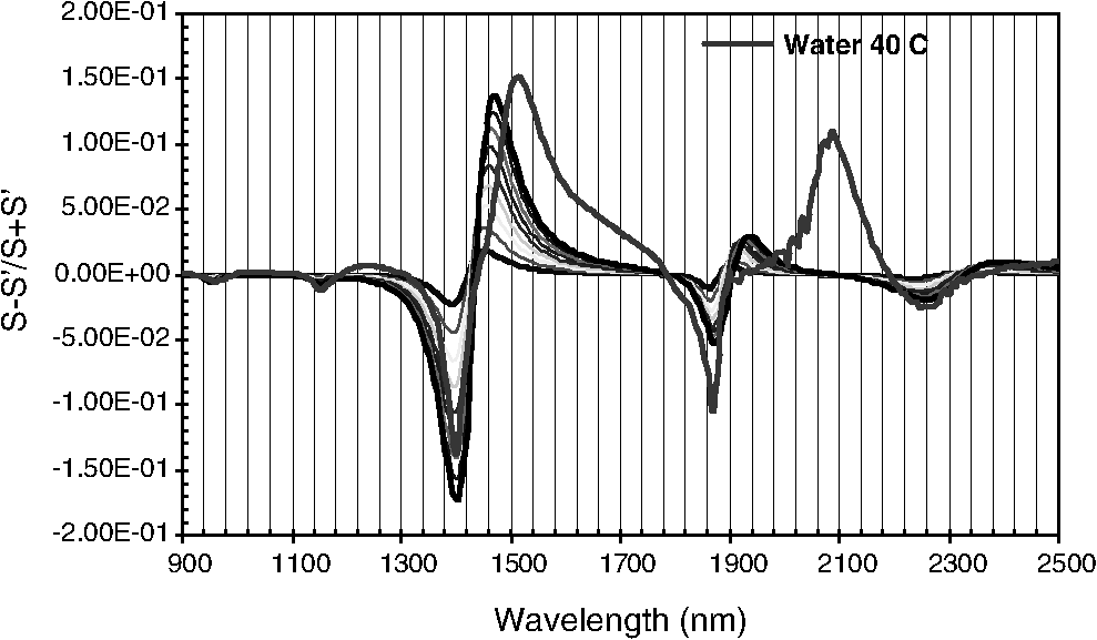$T = 1, \dots, 10$ .

In order to simulate the effect of temperature changes in the spectrum, a linear dependence is assumed with respect to temperature.³² In principle, each of the five absorption bands would have a different rate constant. Since the goal of this article is not to develop a model for water absorption, we have simply assumed that the rate constants are the same for all absorption bands. The values chosen are those that provide a better match to the spectrum and are listed in Table 1.

Defining vectors $B$ and $A$ with components corresponding to a particular pass-band filter as in Eq. (7) and a nonlinear variable, $y (T)$ :

Eq. (23)

B_{i} = \int_{λ_{i} - Δ_{i} / 2}^{λ_{i} + Δ_{i} / 2} E (d, ω) \cdot E^{*} (d, ω) |_{T = T_{0}} \cdot d λ

Eq. (24)

A_{i} = \int_{λ_{i} - Δ_{i} / 2}^{λ_{i} + Δ_{i} / 2} E (d, ω) \cdot E^{*} (d, ω) |_{T} \cdot d λ

Eq. (25)

y (T) = 1 - e^{T / τ},

where the index,

i

, represents a given pass-band of width

Δ λ_{i}

, and

E (d, ω)

is defined in Eq. (22). The parameter

T

is as appears in Table 1, and

τ

is a “critical” value of that parameter. When,

T > \approx τ

, then the expressions for each component,

A_{i}

and

B_{i}

, taken independently, become highly nonlinear.

Figure 17 shows a series of simulated spectra with $T = 0, 1, \dots, 50$ and $τ = 10$ ; the nonlinear nature of the spectral shifts is clear. Superimposed on Fig. 17 is the spectral profile of eight filters with their corresponding set of characteristics ${{(λ_{c}, Δ λ_{c}, κ)}_{1}, \dots, {(λ_{c}, Δ λ_{c}, κ)}_{8}}$ . This particular filter set is such that the expression $S (y)$ is very close to a straight line (see the inset in Fig. 17), where the value of “ $S$ ” is obtained from the filter selection [cf. Eq. (7) in the text]. Figure 17 demonstrates the power of the shell-cloud stochastic routine to produce a linearized outcome, even though the physically meaningful linearity conditions are overwhelmed.

Fig. 17

Simulated water spectra showing a nonlinear profile sequence with respect to a “temperature” parameter, $T$ . The features at 1500 nm are heavily bent toward higher wavelength, as the parameter $T$ is increased. Notice how the dMLR routine selects a filter set, in which weak, inconspicuous features at $\sim 2000 nm$ are weighted more heavily than strong features that become nonlinear more rapidly. The net effect is to produce a linear function, $S (y)$ , shown in the inset. The $R^{2}$ value of the linear fit to $S (y)$ is $R^{2} = 0.9998$ .

Finally, we will briefly review the procedure used to correct for the effect of $T$ fluctuations in the spectral signature of the samples. Figure 18 shows differential spectra of water for temperatures varying from 22 to 40°C. The reference is the water spectrum at 22°C. The inset in the figure shows that the area swept by the spectral features, as they are stretched due to the increase in temperature, follows a linear behavior in the temperature range considered. The ordinates in the inset in Fig. 18 are the integrated area under the absolute value of each spectrum in the figure, as a percentage of the entire area of the spectrum. Since the range of temperature fluctuations in any given data collection procedure never exceeded 2°C, we can safely assume that the impact of these fluctuations is linear. The implication of this is that the effect of temperature and glucose concentration in water can be treated independently.

Fig. 18

Measured relative difference in water spectra at varying temperatures. The inset shows the integrated absolute value of the curves as a function of $T$ (in °C). A linear behavior is obtained. The variance is due to the lower SNR at longer wavelengths.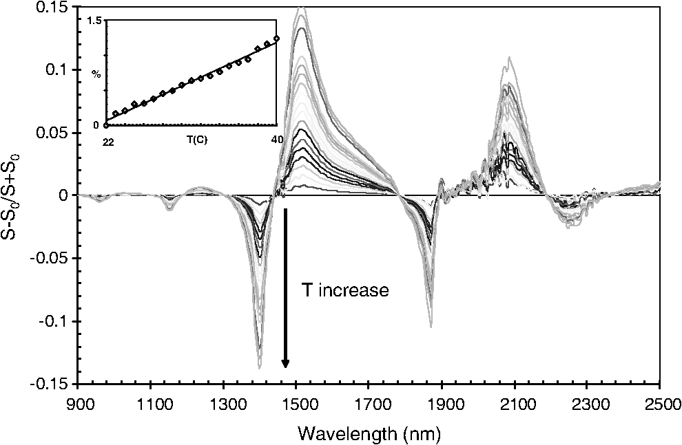

The procedure starts by measuring the temperature, $T$ , at which each glucose spectrum is collected. Then, a water spectrum at temperature, $T$ , is fabricated, $W (λ, T)$ , by using the water spectra at the extreme temperatures, $W (λ, T_{0})$ and $W (λ, T_{A})$ with $T_{0} < T < T_{A}$ , and a reference water spectrum, $W_{ref} (λ, T_{ref})$ , collected at the beginning of every data sampling sequence. The construction of $W (λ, T)$ is taken by assuming a linear stretch between points $T_{0}$ , $T_{A}$ , and $T_{ref}$ :

Eq. (26)

W (λ, T) = \frac{{1 + 2 \cdot ξ \cdot [\frac{W (λ, T_{A}) - W (λ, T_{0})}{W (λ, T_{A}) + W (λ, T_{0})}]}}{{1 + 2 \cdot ξ_{ref} \cdot [\frac{W (λ, T_{A}) - W (λ, T_{0})}{W (λ, T_{A}) + W (λ, T_{0})}]}} \cdot W_{ref} (λ, T_{ref}) .

With the coefficients $ξ$ and $ξ_{ref}$ defined as

Eq. (27)

ξ = \frac{T - T_{0}}{T_{A} - T_{0}},

Eq. (28)

ξ_{ref} = \frac{T_{ref} - T_{0}}{T_{A} - T_{0}} .

With $W (λ, T)$ , the differential spectrum of glucose and pure water at temperature $T$ will only include the effect of glucose in the sample to a linear approximation. This procedure can be implemented with data collected using a grating-based spectrometer using a photodetector array or with an instrument like the one described in this article using architectures as the one shown in Fig. 6.

Acknowledgments

The research project reported in this document was carried out with the generous support of Spencer Trask, Investing Firms of New York, New York.

References

1.

I. Avrutskyet al., “Concept of a miniature optical spectrometer using integrated optical and micro-optical components,” Appl. Opt., 45 (30), 7811 –7817 (2006). http://dx.doi.org/10.1364/AO.45.007811 APOPAI 0003-6935 Google Scholar

2.

TekippeV. J.GuynnR.CarberryJ., “Rotary optical switch,” US Patent Application, Pub. No.: US 2006/0072873 A1 (2006).

3.

E. R. Malinowsky, Factor Analysis in Chemistry, John Wiley & Sons, New York (2002). Google Scholar

4.

M. A. ArnoldG.W. Small;, “Determination of physiological levels of glucose in an aqueous matrix with digitally filtered fourier transform near-infrared spectra,” Anal. Chem., 62 (14), 1457 –1464 (1990). http://dx.doi.org/10.1021/ac00213a021 ANCHAM 0003-2700 Google Scholar

5.

J. ChenM. A. ArnoldG.W. Small;, “Comparison of combination and first overtone spectral regions for near-infrared calibration models for glucose and other biomolecules in aqueous solutions,” Anal. Chem., 76 (18), 5405 –5413 (2004). http://dx.doi.org/10.1021/ac0498056 ANCHAM 0003-2700 Google Scholar

6.

I. Lerche;, “Some notes on entropy measures,” Math. Geol., 19 (8), 843 –852 (1987). http://dx.doi.org/10.1007/BF00893012 MATGED 0882-8121 Google Scholar

7.

C. E. Shannon;, “A mathematical theory of communication,” Bell Syst. Tech. J., 27 379 –423 (1948). http://dx.doi.org/10.1002/bltj.1948.27.issue-3 BSTJAN 0005-8580 Google Scholar

8.

D. W. Allan;, “Statistics of frequency standards,” Proc. IEEE, 54 (2), 2213 –2230 (1966). http://dx.doi.org/10.1109/PROC.1966.4634 IEEPAD 0018-9219 Google Scholar

9.

Y. WangY. WangH.Q. Le, “Multi-spectral mid-infrared laser stand-off imaging,” Opt. Express, 13 (17), 6572 –6586 (2005). http://dx.doi.org/10.1364/OPEX.13.006572 OPEXFF 1094-4087 Google Scholar

10.

K. J. Jeonet al., “Comparison between transmittance and reflectance measurements in glucose determination using near infrared spectroscopy,” J. Biomed. Opt., 11 (1), 014022 (2006). http://dx.doi.org/10.1117/1.2165572 JBOPFO 1083-3668 Google Scholar

11.

G. Yoonet al., “Determination of glucose concentration in a scattering medium based on selected wavelengths by use of an overtone absorption band,” Appl. Opt., 41 (7), 1469 –1475 (2002). http://dx.doi.org/10.1364/AO.41.001469 APOPAI 0003-6935 Google Scholar

12.

X. LiangQ. ZhangH. Jiang, “Quantitative reconstruction of refractive index distribution and imaging of glucose concentration by using diffusing light,” Appl. Opt., 45 (32), 8360 –8365 (2006). http://dx.doi.org/10.1364/AO.45.008360 APOPAI 0003-6935 Google Scholar

13.

W. Chenet al., “Application of transcutaneous diffuse reflectance spectroscopy in the measurement of blood glucose concentration,” Chin. Opt. Lett., 2 (7), 411 –413 (2004). COLHBT 1671-7694 Google Scholar

14.

J. A. TamadaM. LeshoM. J. Tierney, “Keeping watch on glucose,” IEEE Spectrum, 39 (4), 52 –57 (2002). http://dx.doi.org/10.1109/6.993789 IEESAM 0018-9235 Google Scholar

15.

N.V. Iftimiaet al., “Toward noninvasive measurement of blood hematocrit using spectral domain low coherence interferometry and retinal tracking,” Opt. Express, 14 (8), 3377 –3388 (2006). http://dx.doi.org/10.1364/OE.14.003377 OPEXFF 1094-4087 Google Scholar

16.

M. A. ArnoldG. W. Small;, “Noninvasive glucose sensing,” Anal. Chem., 77 (17), 5429 –5439 (2005). http://dx.doi.org/10.1021/ac050429e ANCHAM 0003-2700 Google Scholar

17.

J. Krinsleyet al., “Glucose measurement of intensive care unit patient plasma samples using a fixed-wavelength mid-infrared spectroscopy system,” J. Diabetes Sci. Technol., 6 (2), 294 –301 (2012). Google Scholar

18.

J. T. Olesberget al., “Tunable laser diode system for noninvasive blood glucose measurements,” Appl. Spectrosc., 59 (12), 1480 –1484 (2005). http://dx.doi.org/10.1366/000370205775142485 APSPA4 0003-7028 Google Scholar

19.

V. SaptariK. Youcef-Toumi, “Measurements and quality assessments of near-infrared plasma glucose spectra in the combination band region using a scanning filter spectrometer,” J. Biomed. Opt., 10 (6), 064039 (2005). http://dx.doi.org/10.1117/1.2141934 JBOPFO 1083-3668 Google Scholar

20.

G. YoonS. Hahn, “Identification of pure-component spectra using independent-component analysis in glucose prediction based on mid-infrared spectroscopy,” Appl. Opt., 45 (32), 8374 –8380 (2006). http://dx.doi.org/10.1364/AO.45.008374 APOPAI 0003-6935 Google Scholar

21.

H. M. HeiseA. Bittner, “Multivariate calibration for near-infrared spectroscopic assays of blood substrates in human plasma based on variable selection using PLS-regression vector choices,” Fresenius J. Anal. Chem., 362 (1), 141 –147 (1998). http://dx.doi.org/10.1007/s002160051047 FJACES 0937-0633 Google Scholar

22.

B. R. SollerJ. FavreauP. O. Idwasi, “Investigation of electrolyte measurement in diluted whole blood using spectroscopic and chemometric methods,” J. Appl. Spectrosc., 57 (2), 146 –151 (2003). http://dx.doi.org/10.1366/000370203321535042 JASYAP 0021-9037 Google Scholar

23.

R. Clapset al., “Real-time, broad-band measurement of cholesterol, collagen and elastin using a novel, rotary switch spectrometer,” Proc. SPIE, 6078 60782G1 (2006). http://dx.doi.org/10.1117/12.645345 PSISDG 0277-786X Google Scholar

24.

D. P. Leleuxet al., “Applications of Kalman filtering to real-time trace gas concentration measurements,” Appl. Phys. B, 74 (1), 85 –93 (2002). http://dx.doi.org/10.1007/s003400100751 APBOEM 0946-2171 Google Scholar

25.

R. Clapset al., “Ammonia detection by use of near-infrared diode-laser based overtone spectroscopy,” Appl. Opt., 40 (24), 4387 –4394 (2001). http://dx.doi.org/10.1364/AO.40.004387 APOPAI 0003-6935 Google Scholar

26.

(2008). ttinc.com/download-white-papers Google Scholar

27.

U.S. National Library of Medicine, and the National Institutes of Health, “Comprehensive Metabolic Panel,” (2013) http://www.nlm.nih.gov/medlineplus/ency/article/003468.htm January ). 2013). Google Scholar

28.

E. A. Moschouet al., “Fluorescence glucose detection: advances toward the ideal in vivo biosensor,” J. Fluoresc., 14 (5), 535 –547 (2004). http://dx.doi.org/10.1023/B:JOFL.0000039341.64999.83 JOFLEN 1053-0509 Google Scholar

29.

L. PalchettiD. Lastrucci, “Spectral noise due to sampling errors in Fourier-transform spectroscopy,” Appl. Opt., 40 (19), 3235 –3243 (2001). http://dx.doi.org/10.1364/AO.40.003235 APOPAI 0003-6935 Google Scholar

30.

M. Bradley, “Advantages of a Fourier transform spectrometer,” (2008). Google Scholar

31.

S. Kasemsumranet al., “Selective removal of interference signals for near-infrared spectra of biomedical samples by using region orthogonal signal correction,” Anal. Chim. Acta, 526 (2), 193 –202 (2004). http://dx.doi.org/10.1016/j.aca.2004.09.047 ACACAM 0003-2670 Google Scholar

32.

W. S. PegauD. GrayJ. R. V. Zaneveld, “Absorption and attenuation of visible and near-infrared electromagnetic radiationin water: dependence on temperature and salinity,” Appl. Opt., 36 (24), 6035 –6046 (1997). http://dx.doi.org/10.1364/AO.36.006035 APOPAI 0003-6935 Google Scholar

CC BY: © The Authors. Published by SPIE under a Creative Commons Attribution 4.0 Unported License. Distribution or reproduction of this work in whole or in part requires full attribution of the original publication, including its DOI.

Citation Download Citation

Ricardo Claps and Jeffrey Virojanapa "Fast, broadband, rugged spectrometer for near-infrared measurements of organic solutions and multicomponent mixtures," Journal of Biomedical Optics 18(11), 117001 (1 November 2013). https://doi.org/10.1117/1.JBO.18.11.117001

Published: 1 November 2013

Access the abstract

JOURNAL ARTICLE
13 PAGES

DOWNLOAD PAPER SAVE TO MY LIBRARY

GET CITATION

CITATIONS

Cited by 1 scholarly publication.

Explore citations on Lens.org

KEYWORDS

Glucose

Absorption

Spectroscopy

Near infrared

Water

Clouds

Calibration

1.

Introduction

2.

Discrete Multivariate Linear Regression Analysis