1.

Introduction

The light property chosen in this study to highlight imaging contrast is the polarization, as proposed by Tuchin,^1,2 Jacques et al.,³ Angelsky et al.,⁴ and Guyot et al.⁵ In fact, it provides a good fingerprint of the substructure of a medium since the depolarization is the most important scattering effect in comparison to dephasing and simple attenuation.^6,7 As introduced, the DOP technique allows enhancement of many structural details that are often impossible to differentiate with naked eye and/or classical imaging methods. Classical techniques carry out mainly the intensity differentiation, as suggested by Ghosh and Vitkin,⁸ Ramell-Roman et al.,⁹ and Garcia et al.¹⁰ In our case, we complete these approaches by the possibility of imaging all the possible polarization (linear, circular, but also elliptic ones).¹¹ Moreover, the medium characteristics can be achieved by the system multispectral capability and in near real time.

Let us consider the Mueller formalism in Sec. 2 to introduce our purpose. Considering the system presented in Sec. 3, its validation will be demonstrated through several test media in “transillumination mode.” Thus, a complete chart will be obtained with a set of resulting images as a function of the polarization input. All these results will be the subjects of Sec. 4.1. Section 4.2 is devoted to the second validation part, which will consider the system in backscattering configuration for several test media.

To conclude, an example of dynamical monitoring of a biological sample will be shown in the end of Sec. 4.2, followed by discussion and perspectives in Sec. 5.

2.

Theory: Mueller–Stokes Formalism and DOP Methods

The system captors are two charge-coupled diode (CCD) cameras, so the acquired images correspond to the scattered polarized intensities. In this case, the corresponding mathematical model has been proposed by Stokes and Mueller;^12,13 while the first one is a vectorial description based on measurable intensities, the second one is related to the changes of these same Stokes intensity vectors after the interaction of the light with a medium. In fact, a real element square Mueller matrix (MM) of range four is associated to the sample and defined as

Thereby, considering Mueller’s theory, the complete system, showed in Fig. 1, can be described by product of the Stokes vector $S$ associated to the input beam for the Mueller matrices associated to each optical component. As a consequence, the intensity vector $S^{\prime \prime }$ coming out from the proposed optical system is easily described by the following relationship:

Fig. 1

Schematic diagram of the experimental system: the illumination part (halogen white lamp, L₁ aspherical condenser, color filters), the polarization state generation (PSG) (LP, linear polarizer; ${\mathrm{LCVR}}_1$, light crystal variable retarder), the sample location for the scattering medium, the polarization state analyzer (PSA) (${\mathrm{LCVR}}_2$ and BS polarized beam splitter cube) and the detection system (${\mathrm{CCD}}_1$ and ${\mathrm{CCD}}_2$ cameras).

Introducing the dependence by the matrices associated to each component:

At this point, the definition of the degree of polarization (DOP) has to be introduced

It is really important to keep in mind that the both perpendicular components ($I_{\parallel }$ and $I_{\perp }$) of a beam can be linear, circular, or elliptic too and not only linear polarization in both directions.

Hence, when the sample is known, i.e., the associated matrix MM, the last parameter for DOP is the LCVR retardance $\delta$, which in turn is a function of the applied LCVR voltage. Let us remark that for zero retardance, the DOP degenerates in the linear one, whereas $\delta =\pi /2$ is the case for the circular DOP. Between the both, the ellipticity can be easily controlled.

Another detail to be considered is one other experimental condition. The system has been conceived in backscattering condition, with an angle of 15 deg between the incident and the reflected beam, in order to prevent specular reflection on the medium and therefore imaging artifacts.³ We assume that this angle will be neglected in the following cases.

3.

Materials: Experimental System

The schematic layout of the proposed experimental system is shown in Fig. 1: the illumination part, the polarization state generation (PSG), the sample location, the polarization state analyzer (PSA), and finally the detection system.

A halogen lamp (Olympus, Tokyo, Japan, CLH-SC 150 W) is focused using an aspherical system composed of an aspherical condenser $L_1$ (LA 1027, Thorlabs, Maisons-Laffitte, France, $f_1=35\mathrm{mm}$) and then comes out from a fiber bundle and passes through two color filters $L_2$ and $L_3$. Therefore, $L_1$ provides a quasi homogeneous spot over all the field of view, to prevent the beam having a Gaussian profile. For the same reason, if necessary, also a ground grass diffuser (DGK01, Thorlabs) can be interposed between $L_3$ and the following LP. On the other side, $L_2$ and $L_3$ are used to adapt light spectra ranges with the used CCD cameras. In particular, this range between 500 and 720 nm corresponds with the well-known “therapeutic windows,” which in case of biological media is the most considered.

At this point, the polarization state is fixed using the PSG composed of a LP (LPVIS-100MP, Thorlabs), whose transmission axis defines the polarization axes of the system; it is followed by the first nematic liquid crystal variable retarders ${\mathrm{LCVR}}_1$ (LCR-1-VIS, Thorlabs). This last is oriented at 45 deg to the LP polarization axis and is remotely controlled by a power supply (LCC25, Thorlabs). The nematic liquid crystal is an optical component based on birefringent behavior which introduces phase retardance between the two Cartesian projections of the electric beam. By that, it changes the ellipticity of the beam as well as its polarization. Thus, just changing the voltage applied to the lens windows, it allows the generation of all the feasible polarizations, preserving the multispectral information.

Thence, after the interaction with the sample, light reaches the PSA, which is composed of the second ${\mathrm{LCVR}}_2$, coupled in charge and orthogonal fast axis with the first one and so at $-45\mathrm{deg}$ to LP polarization axis. Due to its important role, the LCVRs calibration has been verified, in terms of retardance as a function of the applied voltage, as explained in the next section. Moreover, as demonstrated in Fig. 1, there is an angle of 15 deg between the optical PSG axis and the PSA axis, which prevents specular reflection on the medium and so imaging artifacts.³

Finally, the beam reaches the polarized splitter cube (BS), which separates the two perpendicular components of the output intensity captured by both cameras.

Note that the whole system is remotely controlled by a routine in MATLAB with Software Development Kit (SDK) function. In particular, the operator can change the exposure time to avoid the CCD saturation according to the reflectivity of the sample and the introduced retardance.

4.

Materials: Measurement

Some general characteristics of the acquired images will be presented, such as the sequence of the experimental calibration and validation tests.

The proposed measurements are executed as a function of the retardance, so each series proposes an RGB image for each value of imposed retardance. For this reason, the calibration of the retardance as a function of the incident wavelength has been verified for each liquid crystal. In particular, it has been tested that three different applied tensions are necessary to obtain the same polarized state coming out from the LCVR for each one of the three captured intensities, such as for each CCD channel capture. As a consequence, whereas the commutation time of the LCVR and the functioning of the CCD cameras, near $12\text{images}/\mathrm{s}$ will be captured; for this, the system is regarded as near real time. The retardance will be considered in a range between 0 and $0.5/\pi$. It allows linear, elliptic, and circular polarizations without any redundancies.

To proceed with the evaluation, a region of interest (ROI) is selected corresponding to the minimal flux in the background image of $I_{\perp }$ acquired with no light. After that, for each image, the corresponding ROI of the dark background image is subtracted pixel by pixel and, since the captured image is an RGB one, the result will be transformed in grayscale, to obtain a corresponding two-dimensional matrix for the final calculations.

From the evaluation of the behavior of the beam splitter, a difference between transmission and refractive coefficient has been observed during these calibration measurements. For this reason, a ratio of normalization is necessary with respect to a blank image captured using a nonpolarized white light source. It is calculated pixel by pixel between both CCD cameras and it will be multiplied for each image. Next subsections propose the validation measurement in transmission and in backscattering mode observed in near real time.

4.1.

Transmission Calibration Measurement

Initially, the setup will be considered in transmission mode and the schema proposed in Sec. 3 is modified as in Fig. 2.

Fig. 2

Outline of the first system used for the validation measurement in transmission condition, in particular, the LCVR is oriented at $\pm 45\mathrm{deg}$ to the polarization axis imposed by LP.

First, verification regards the transmission of the two LCVRs for the same retardance: two series will be captured for a system composed of the illumination focused source, the LP, one of the two liquid crystals with its own orientation ($+45\mathrm{deg}$ for ${\mathrm{LC}}_1$ and $-45\mathrm{deg}$ for ${\mathrm{LC}}_2$), which play the role of samples and the detection system. As shown in Fig. 3 and in agreement with the Mueller calculus [see Eq. (3) and Fig. 3(b)], it is checked that the total captured intensity remains constant, since the total flux remains the same, while the difference of the two ($I_{\parallel }-I_{\perp }$) will decrease with the same behavior for the two crystals. More than that, as predicted by the scattering theory,⁶ for nonlinear polarization and considering multiple scattering interactions, $I_{\perp }$ changes more than $I_{\parallel }$. Here, as in the following, the evaluation of the results is just qualitative because a complete characterization requires more detailed studies and it is not the aim of this article. Moreover, it is really important to keep in mind that $I_{\parallel }$ and $I_{\perp }$ are not the classical notations of linear polarizations but the both perpendicular components of an output polarized beam on the CCD detectors in which polarization can be linear, circular, or elliptic too.

Fig. 3

(a) The graph shows the difference (dotted line) and the sum (solid line) using ${\mathrm{LVRC}}_1$ and ${\mathrm{LVRC}}_2$ (square markers). (b) The same curves are obtained from Mueller calculus: sum (continuous) and difference (dotted) of the intensities for ${\mathrm{LVRC}}_1$ and the same for the superimposed square (for sum) and circle (for difference) markers considering ${\mathrm{LVRC}}_2$.

Experimental versus theoretical behavior of the LCVR may be compared in Fig. 4.

Fig. 4

The degree of polarization (DOP) resulting by (a) measurement for the ${\mathrm{LCVR}}_1$ (continuous line) and ${\mathrm{LCVR}}_2$ (dashed line with square markers); and (b) simulation in ideal conditions: continuous line ${\mathrm{LCVR}}_1$ and square markers for ${\mathrm{LCVR}}_2$.

To complete the calibration tests, three other media were imaged: no sample, a homogeneous absorber (a color filter), and a so-called diattenuator, i.e., an LP. An example of the obtained images is shown in Fig. 5.

Fig. 5

Practical demonstration of the correct behavior of the system, an example of the images acquired for an imposed retardance of $0.05/\pi$, such as linear incident state. The first image corresponds to $I_{\perp }$, while the second is $I_{\parallel }$. As expected, all the intensity is collected by the first CCD since it corresponds to the parallel flux $I_{\parallel }$; as a consequence, the perpendicular flux $I_{\perp }$ corresponds to a quite dark image. The third image is DOP one.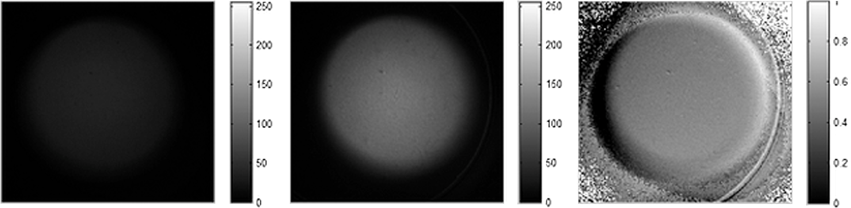

Considering the first two cases, they differ just for a reduction by a constant factor linked to the absorption, given that the polarization is not modified. On the counterpart, for both, the intensity detected by ${\mathrm{CCD}}_1$ has to be maximal, while the flux on ${\mathrm{CCD}}_2$ has to be almost null as shown in Fig. 6. Thus, it has been verified that the total flux remains quite constant. Moreover when, using the first LP, the input incident imposed polarization is linear and there is no sample which can modify this state; all the intensity is detected by ${\mathrm{CCD}}_1$, while on ${\mathrm{CCD}}_2$, a quasi-zero image is done to a residual transmittance of the cube, also for the perpendicular polarization. Note that, for all the possible incident polarization state, theory is in agreement with our experimental results.

Fig. 6

Considering no sample, the intensities as a function of the retardance is shown: the continuous line with circle markers corresponding to $I_{\parallel }$ and detected by ${\mathrm{CCD}}_1$ and the other continuous line with diamond markers is $I_{\perp }$ since detected by ${\mathrm{CCD}}_2$. The others lines correspond to the sum (continuous) and difference (dashed) of the intensities.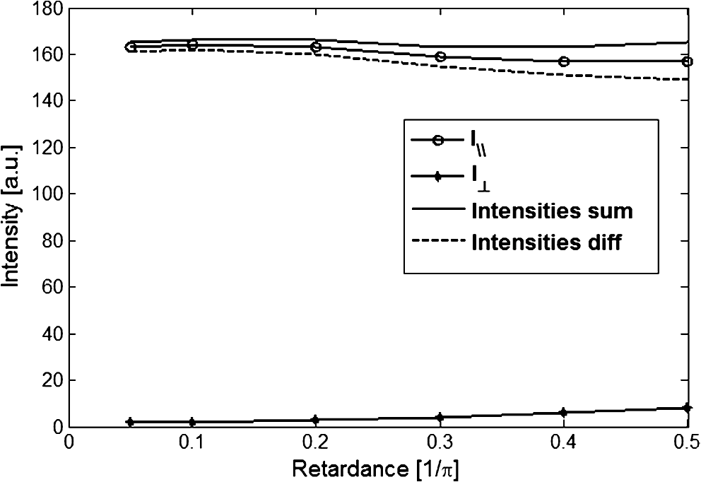

Accordingly, the DOP for this system has to be constant and near 1. As expected and shown in Fig. 7, the DOP curves follows a quite ideal behavior of the system, the resulting DOP mean is $0.95\pm 0.01$ in the first case considering the complete setup, while the DOP is $0.88\pm 0.01$ when the sample is the color filter. The two cases shows that the losses are linked to the transmission and refraction indices of the two media, for example a larger absorption and so the reduction of the DOP.

Fig. 7

Calculated DOP for the system with no sample and considering a color filter, for this example a blue one; in the first case, the mean value is $0.95\pm 0.01$ (continuous line) and for the other one is $0.88\pm 0.01$ (dashed line).

With respect to the filtering effect, the LP has been used in two perpendicular configurations. As a consequence, in this case (see Fig. 8) also, the total flux will decrease since a part of the incident flux is eliminated before the interaction with the sample with no connection with depolarization.

Fig. 8

Comparison of the intensities acquired considering LP at 0 deg; $I_{\parallel }$ (continuous line with circle markers) and $I_{\perp }$ (continuous line with diamond markers) correspond to both perpendicular components of the beam while the other are their sum (continuous) and their difference (dashed).

In fact, when LP sample is at 0 deg and the incoming polarization is linear, the total intensity is detected by ${\mathrm{CCD}}_1$; after increasing the retardance, incoming linear polarization becomes progressively elliptic and finally circular, $I_{\parallel }$ has to reduce and $I_{\perp }$ increase, since two phenomena have to be considered: the flux passed after the LP decreases because of the filtering effect of the sample and $I_{\perp }$ is more scattered than $I_{\parallel }$¹⁴. The obtained DOP is shown in Fig. 9. Inversely for LP at 90 deg, there is no intensity propagating through the system, so the images are quasi-zero values. To note a residual refraction of the beam splitter for zero retardance when a zero refracted intensity is still observed, in fact $I_{\perp }$ is not zero for retardance equal to $0.05/\pi$.

Fig. 9

Calculated DOP for LP at 0 deg.

Furthermore, the experimental calibration results in “transillumination” mode that agrees with the simulated behavior done using the Mueller formalism, and thus the complete validity of the method is demonstrated.

4.2.

Backscattering Calibration Measurements

Now, the final evaluation of the results of the complete system will be discussed and some preliminary images presented.

The same series of measurements described in the previous subsections are executed in backscattering mode as considered in Fig. 1. Following that calibration method, a polarimetric mirror will be considered as homologous of no sample. In any case, keep in mind that these mirrors are largely imperfect due to their rugosity. After that, it will be the case of the LP and finally, the homogeneous scattering media, such as a cloth of black velvet or white sheet of paper, for simple absorption with homogeneous scattering of different densities and hence depolarization.

On the counterpart, the subject of the preliminary medical test is a hand, taking into account a video showing the evolution of the interaction between polarized light and complex biological medium.

In the case of both metallic plates with different rugosities, the expected results are presented in Fig. 10. It gives a DOP of about $0.42\pm 0.04$ for the first sample and about $0.78\pm 0.01$ for the second one. The reduction of the mean values with respect to 1 is linked to the rugosity of the used metallic plate. Thus, the correct system response has been verified since the curve is constant.

Fig. 10

DOP for the two examined polarimetric mirrors; as expected, they are constant.

The DOP for the LP follows the same case in transmission mode (Fig. 11 to compare with Fig. 9) as predictable. Even in this case the initial maximum is not 1, as its homologous in transmission mode; on the other hand, the presence of a negative $\mathrm{DOP}=-0.05\pm 0.01$ can be interpreted as an offset due to the BS characteristics, in particular to the wavelength dependencies of the refraction index.

Fig. 11

DOP obtained when the sample is a LP.

The last executed tests demonstrate the agreement with the case of no sample and color filter. The results are shown in Fig. 12, where the samples are black velvet and a blank sheet of paper. Let us remember that the second one is denser and as a consequence more depolarizing, hence the DOP will be lower.

Fig. 12

The DOP calculated in the case of black velvet (continuous line) and white paper sheet (dashed line).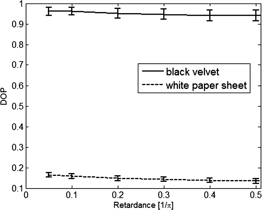

These studies are important because they verify the different responses in case of media corresponding to different densities, i.e., concentration.

Finally, the last snaphshot of the video of a chosen area of the dorsum of the hand (Fig. 13) shows the result for retardance equal to $0.2/\pi$ in color scale; this has been used to enhance the difference related to distinct penetration deeps associated to the interacting bandwidth wavelenght, i.e., the three CCD channels.

Fig. 13

Snapshot of the proposed video where the sample is the dorsum of the hand, in order from left to right and top to bottom: the RGB complete image and then the pure color images: red, green, and blue. Each image corresponds to the same chosen zone, for retardance equal to $\mathrm{Ret}=0.2[1/\pi ]$ (shown in the top left corner of each image in units of [$1/\pi$]); the color scale is fixed (Video 1, MPEG, 7.4 MB) [URL: http://dx.doi.org/10.1117/1.JBO.18.11.116002.1].

This last proof shows the evolution as a function of the input polarization state. It is a promising prospective for future medical application.

5.

Conclusion

In this article, we propose a new noninvasive, noncontact dynamic imaging technique. This experimental setup allows the near-real-time multispectral acquisition of the so-called “DOP” in polarimetry preserving the spectral information. This DOP can be obtained with controlled ellipticity (from linear to circular one) and as such, it is possible to fully characterize a complex biological medium enhancing its characteristics. This method is not conventional according to more traditional techniques and due to the peculiar use of the dynamic variation of the input beam polarization allowed by the liquid nematic crystals, it improves the comprehension of the light-matter interaction using the depolarization as index.

Therefore, further works will be devoted to a better understanding of the scattering phenomena in biological tissues, and more precisely in the particular case of the several ellipticities of the incoming beam. Moreover, the dependencies with the wavelength will be also explored. To this aim, we actually start a study in dermatology on the so-called sickle cell where the publication of this polarimetric setup will be the first step.