1.

Introduction

Second harmonic generation (SHG) imaging has emerged as a powerful tool for imaging biological tissues with submicron resolution and promises future potential for in vivo clinical applications.¹ SHG has been observed in both forward and backward detections from collagen fibers in structural protein arrays and acto-myosin complexes in muscle.² For in vivo imaging of thick samples, backward SHG is the only possible signal source. Therefore, it is of importance to understand the mechanism of backward SHG. The SHG initial emission pattern is related to the size of the scattering objects. Small scatters, i.e., much smaller than the excitation wavelength, produce a “figure 8” spatial pattern.³ When the adjacent molecules form aligned structures comparable to or larger than the excitation wavelength in the axial direction, the emission becomes highly forward generated. Efficient backward generation does not happen unless the aligned structures satisfy a certain periodic structure so that the backward generations from multiple entities are constructively interfered with each other.⁴ If the sample is thick or the scattering coefficient is large, the backscattering of the forward generated SHG might become a source of backward SHG that is not negligible.

In this paper, we investigate the SHG signal from tissues at forward and backward directions. It is helpful to clearly define the SHG components collected by detectors in both directions. In Fig. 1, the SHG initiated from the focal point is named as forward generated SHG and backward generated SHG (BG-SHG) according to their generation direction. Due to the existence of tissue scattering, the forward generated SHG might be backscattered and is named as backward-scattered forward-generated SHG (BS-SHG). The total SHG collected in the backward direction, consisting of BG-SHG and BS-SHG, is simply named as backward SHG (B-SHG). Similarly, in the forward direction, we have forward-scattered backward-generated SHG and forward generated SHG.

Fig. 1

An illustration of photon generation and collection by pinholes in the Monte Carlo simulation with various second harmonic generation (SHG) signal components in forward and backward directions.

Previously, we investigated the wavelength dependency of SHG from 10 μm thick mouse tail tendon tissues. In addition to the observation that the SHG intensity decreased from shorter to longer excitation wavelength, it was found that similar wavelength dependency appeared in both forward and backward directions.⁵ Recently, we observed the same phenomenon from various collagen tissues with 100 to 300 μm thickness (data not shown). An interesting question is the origin of this similar wavelength dependency in two directions, which is closely related to the generation mechanism of forward and backward SHG. Quantifying the backward scattering of SHG from tissues may help to understand the origin of this phenomenon.

For understanding the issue of SHG signal scattering in tissues, it is interesting to study the contribution of BS-SHG among the B-SHG. Campagnola et al. qualitatively investigated this issue in cellulose specimens.⁶ It was observed that from depths near the tissue surface, the backward channel displayed small fibrils not present in the forward channel. In addition, at depths beyond one mean free path of scattering, the fibril morphologies became highly similar, suggesting the observed backward contrast was also composed of a component that arose from multiple scattering of the initially forward generated signal. In the entire 500 μm thickness of the cellulose, the ratio of forward SHG over backward SHG intensity (F/B) increased from unity to 6.2. It was explained that when the excitation focal point was moved deeper into the sample, the backward generated SHG became less coherent due to enhanced scattering, causing the backward signal to decrease. The forward generated SHG experienced less scattering because it was approaching the bottom surface of the tissue, causing the forward signal to increase. Although the trend of image composition variation along the depth is known through these investigations, to the best of our knowledge, there is no quantitative analysis about the variation of BS-SHG and BG-SHG among the B-SHG.

As an attempt to quantify the contribution of BS-SHG to the B-SHG, Legare et al. measured the proportion of BS-SHG to the forward generated SHG in the mouse Achilles tendon and fascia.⁷ The B-SHG from thick samples was compared to the B-SHG from thin samples. This measurement, together with the F/B ratio obtained from thin samples, determined the proportion of BS-SHG to the forward SHG, which was 20 and 2% for 2-mm thick mouse Achilles tendon and fascia tissues, respectively. In Ref. 7, the F/B ratios for tendon and fascia from 10 μm tissue samples were measured to be 25 and 4.2, which implied that the BS-SHG accounted for 83 and 44% of the B-SHG, respectively. According to Legare’s measurements, the BS-SHG dominated the B-SHG in a 2-mm thick mouse Achilles tendon, while it contributed equally to the B-SHG with the BG-SHG in fascia tissues a few millimeters thick.

Compared to the previous quantitative studies, our study extends extensively from two aspects. First, the contribution of BS-SHG to the B-SHG and the proportion of BS-SHG among the forward SHG are quantified and compared from collagen tissues in various conditions, such as at different tissue depths, with different scattering coefficients, and different thicknesses. These experimental results are in good agreement with Monte Carlo (MC) simulation. Second, a pinhole method is presented to quantify the contribution of BS-SHG and BG-SHG to the B-SHG. One advantage of this method is that the proportion of BG-SHG and BS-SHG among the B-SHG can be calculated without the need of forward detection, which can be useful for potential clinical applications.

Previously, Han et al. presented a similar method to measure the F/B ratio without using a forward detection channel in a confocal multiphoton microscopy.⁸ The authors separated the BG-SHG and BS-SHG according to their distinct spatial distribution of signal intensity in the confocal pinhole plane. The BG-SHG was described as a Gaussian distribution with a narrow peak when the scattering after generation was neglected, while the BS-SHG was described as a uniform distribution over the radial distance from the optical axis due to its diffusive nature. Their summation constituted B-SHG in the pinhole plane. The relative amplitudes of the Gaussian and uniform distributions were obtained by collecting the B-SHG through a series of pinholes of different radii, and these relative amplitudes were converted to the proportion of BS-SHG to B-SHG. However, their method has only been applied to a focal depth near the surface. In this paper, we will extend the method to a more general condition where the focal depth is not limited to the surface and also consider scattering of the BG-SHG.

In this paper, we apply the model of SHG signal distribution described in Ref. 8 and extend the SHG pinhole measurement based on various core-diameter fibers in a confocal multiphoton microscopy to investigate the proportion of BS-SHG to the forward generated SHG and the B-SHG from different mouse collagen tissues. In Sec. 2, the pinhole measurement methods to quantify BS-SHG and BG-SHG are described and validation by MC simulation is given in Sec. 3. Further discussions about how various factors, such as depth, scattering coefficient, and thickness affect the scattering performance are presented in Sec. 3 as well. Experiments conducted on two kinds of mouse collagen tissues-mouse tail tendon and Achilles tendon—for measuring the backward scattering of SHG under various conditions such as different depths, scattering coefficients, and tissue thicknesses are presented in Secs. 4 and 5. The perspective of understanding SHG generation is also briefly discussed in Sec. 5.

2.

Methods

3.

Monte Carlo Simulations

In order to characterize the distribution of BG-SHG and BS-SHG in the pinhole plane and to validate the pinhole method, an MC simulation is conducted. The purpose is to examine the BG-SHG spatial distribution on the pinhole plane when the focal point is not on the surface but inside the tissue. This is necessary because only if its distribution satisfies the Gaussian expression can we apply multiple pinhole measurements and curve fitting with Eq. (4). When the scattering is too strong, the BG-SHG distribution may deviate from Gaussian expression, which may affect the accuracy of the pinhole method. In Ref. 8, the authors assumed that the focal point was close to the top surface and the BG-SHG was Gaussian distributed. Therefore, their measurements were restricted to the surface only. Another requirement of applying Eq. (4) is the uniform distribution of BS-SHG intensity in the pinhole plane. For thin tissue samples with small scattering coefficients, the uniform distribution may not be satisfied. Besides examining the BS-SHG and BG-SHG distribution under various conditions, BS-SHG and BG-SHG photons can be differentiated by MC simulation so that the contribution of forward SHG and B-SHG can be obtained. Comparing these results with the ones obtained from the simulating pinhole method, the principle of the pinhole method can be validated.

As a confocal setup, pinholes with various radii are used to collect the photons as shown in Fig. 1, where the pinhole plane is conjugate to the focal plane (pinhole image plane). The magnification from the objective and focus lens pair is set to be unity in our simulation for simplicity. Photons generated at the focal plane need to propagate through the tissue and pass through the pinhole prior to being collected. If the BG-SHG is generated at the tissue surface, then tissue scattering in the collection path can be neglected and the signal spot size at the pinhole plane should be the same as the signal spot size at the focal plane. However, if the BG-SHG is originated from deeper inside the tissue, then the signal spot size at the pinhole plane should be much larger than the signal spot size at the focal plane due to scattering. Effect of scattering on the signal spot size at the pinhole plane can be simulated by MC.

Only the photons that fall within the pinhole and the collection angle of the detection system will be collected. Each photon exits the tissue surface at a specific position and angle, which link a unique ray trace between the pinhole plane and the pinhole image plane. Therefore, when an SHG photon exits the tissue, it is geometrically back-projected to the pinhole image plane, where it can be analyzed to determine whether it falls within the image of the confocal aperture on that plane and, thus, can be collected by the optical system or not.⁹ For example, the photon following the blue path in Fig. 1 is not collected by the pinhole, but the photon following the green path is collected. Other than the position of the back-projected photon, its exit angle with respect to the optical axis needs to be smaller than the NA of the objective lens in order to be collected. The interface between cover glass and collagen tissue does not alter the SHG ray path because the refractive index of collagen at 400 nm is close to that of glass,¹⁰ while the interface between the cover glass and immersion water is supposed to bend the SHG ray path slightly away from the optical axis due to their relative refractive indices. However, it does not affect the conjugate nature between the pinhole plane and its image plane. Due to the conjugate relation between the pinhole image plane and the pinhole plane, the distribution of SHG signal on the pinhole plane can be plotted according to the distribution on the pinhole image plane determined by this back-projection method.

As the general formalism of the MC simulation has been presented in detail by Wang et al. in Ref. 11, we only report the modification to the basic approach required to simulate the propagation of the forward and backward generated SHG photons. In the simulation, 800-nm excitation wavelength and an objective lens with $\mathrm{NA}=0.8$ are used. The forward and backward generated SHG photons have a Gaussian distribution at the focal plane with ${\omega }_0=0.5\mu \text{m}$, according to the $1/e^2$ width of the lateral intensity squared profile ${\omega }_0=0.325\lambda /(1.4{\mathrm{NA}}^{0.91})$.¹² The angle distribution of the SHG photons cannot be simply determined by the NA of the objective lens because the phase matching condition refrains a large angle emission from happening. Therefore, we use the experimentally measured parameters given in Ref. 8 as $\theta =\pm 15\mathrm{deg}$ around the optical axis as the maximum emission angle from the optical axis. The refractive index of the tissue and the water surrounding the tissue are 1.5 and 1.3, respectively. The anisotropy, scattering, and absorption coefficients are 0.9, $150{\mathrm{cm}}^{-1}$, and $1{\mathrm{cm}}^{-1}$ unless otherwise stated.^13,14 The reduced scattering coefficient ${\mu }_s^{\prime }=15{\mathrm{cm}}^{-1}$ is within the range of measured values in Ref. 15.

Figure 2(a) plots the intensity distributions of BG-SHG, which are generated at different depths, over the radial distance from the optical axis. The tissue is modeled as 300 μm thick. All the intensities are normalized to their maximum at optical axis. It is observed that BG-SHG generated at 50, 75, and 100 μm depths decays exponentially with the radial distance from the optical axis and the half widths at $1/e^2$ are 5.0, 8.2, and 13.0 μm, respectively. The deeper the focal plane, the larger the spot size of the BG-SHG observed at the pinhole image plane due to increased scattering. At these depths, the distributions of BG-SHG match with the Gaussian shape. As a comparison, the distribution of BG-SHG in a sample as thin as 10 μm from which the scattering effect can be neglected is plotted in Fig. 2(b). Without scattering, the width of the SHG spot is not broadened in the pinhole image plane so that it keeps the same half width of the original focal spot as 0.25 μm.

Fig. 2

(a) The backward generated SHG (BG-SHG) intensity versus radial distance from optical axis in the pinhole image plane for SHG at 50, 75, and 100 μm depth. (b) BG-SHG intensity distribution without scattering in the pinhole image plane. (c) Backward scattered forward generated SHG (BS-SHG) intensity versus radial distance from optical axis at 50 μm depth with 300 μm thicknesses; (inset) the zoomed in BS-SHG distribution over a shorter range. (d) Dependence of relative backward collected SHG (B-SHG) power on pinhole sizes for F/B  $\mathrm{ratio}=7.5$ in the focal plane at the 50, 75, and 100 μm depths. (e) BG-SHG intensity versus radial distance from optical axis for reduced scattering coefficients 15, 45, and $75{\mathrm{cm}}^{-1}$. (f) Dependence of relative B-SHG power on pinhole sizes for F/B  $\mathrm{ratio}=7.5$ in the focal plane at three reduced scattering coefficients. (g) BS-SHG intensity versus radial distance from optical axis for tissue thicknesses as 300, 500, and 1000 μm. (h) Dependence of relative B-SHG power on pinhole sizes for F/B  $\mathrm{ratio}=7.5$ in the focal plane for the three thicknesses.

Figure 2(c) shows the distribution of BS-SHG in the pinhole image plane. Due to multiple scattering, the BS-SHG has a very broad spot size. It is relatively uniform within 100 μm and then starts to decrease exponentially when the radial distance is $>100\mu \text{m}$ as shown in the inset of Fig. 2(c). The fluctuation is due to the limited number of photons simulated in the simulation.

We then draw the dependence of B-SHG power on the pinhole size, assuming the ratio of forward and backward generated SHG is 7.5 in the focal volume at 50, 75, and 100 μm focal depths as shown in Fig. 2(d). This particular ratio is from mouse tail tendon $\mathrm{F}/\mathrm{B}$ intensity ratio experiment measurements, which will be described in Sec. 5. Good model fittings are obtained when $\omega =5\mu \text{m}$ and $fc/b=0.0003$ for the 50 μm focal depth, $\omega =8.2\mu \text{m}$ and $fc/b=0.00075$ for the 75 μm focal depth, and $\omega =13\mu \text{m}$ and $fc/b=0.0018$ for the 100 μm focal depth. From the $\omega$ and $fc/b$ values, the $\rho$ and $c$ parameters are obtained as $\rho =19.4\%$ and $c=3.2\%$ for 50 μm depth, $\rho =18.4\%$ and $c=3.0\%$ for 75 μm depth, and $\rho =17.4\%$ and $c=2.8\%$ for 100 μm depth, respectively. It shows that the deeper the focal depth (with fixed tissue thickness), the less BS-SHG contributes to the backward SHG. Since the path length for the generated photons is shorter when the depth is deeper, the BS-SHG photons are less likely to be backscattered. The results obtained by this method are compared with MC simulation. In the simulation, we differentiate the BS-SHG and BG-SHG photons collected within the 100 μm radius area in the pinhole image plane according to their original generation direction. The simulation gives $\rho =19.9\%$ and $c=3.2\%$ for 50 μm depth, $\rho =16.8\%$ and $c=2.7\%$ for 75 μm depth, and $\rho =15.6\%$ and $c=2.4\%$ for 100 μm depth. The good matching between simulation and our fitting method validates the principles of this pinhole measurement in the above conditions.

The scattering properties of tissues may vary over a large range among different tissue types and species. Therefore, we also simulate the intensity distribution of BG-SHG at 50 μm depth with reduced scattering coefficient ${\mu }_s^{\prime }$ of 15, 45, and $75{\mathrm{cm}}^{-1}$ in a 300-μm thick tissue as shown in Fig. 2(e). A reduced scattering coefficient of $45{\mathrm{cm}}^{-1}$ approximates that of the Achilles tendon, which is a tissue type measured in our experiment and in Ref. 7. The spot size increases from 5 to 30 μm and a Gaussian distribution is still observed with the scattering coefficient increased from 15 to $45{\mathrm{cm}}^{-1}$. However, when the scattering coefficient increases to $75{\mathrm{cm}}^{-1}$, the BG-SHG shows a $1/e^2$ half width of $\sim 88\mu \text{m}$, but the shape deviates from a Gaussian distribution.

The dependence of B-SHG on pinhole size is simulated in Fig. 2(f) with the above scattering coefficients. The F/B intensity ratio is still 7.5. Substituting the $\omega$ obtained in Fig. 2(e) into Eq. (4), the optimum model fitting are obtained with $fc/b=0.0003$, 0.021, and 0.45 for the reduced scattering coefficients of 15, 45, and $75{\mathrm{cm}}^{-1}$. The corresponding $\rho$ and $c$ are 21.2 and 3.5%, 34.2 and 10.5%, and 59.0 and 20.5% for 15, 45, and $75{\mathrm{cm}}^{-1}$. Direct MC simulation results are 19.9 and 3.2%, 32.1 and 10.2%, and 53.0 and 17.1%, respectively. The difference between pinhole method and simulation increases with ${\mu }_s^{\prime }$, such as the ${\mu }_s^{\prime }=75{\mathrm{cm}}^{-1}$ case. For large ${\mu }_s^{\prime }$, since $\omega$ deviates from Gaussian, the $fc/b$ parameters have to be set higher for good fitting, which results in an overestimation of the BS-SHG. It demonstrates that our pinhole measurement method has a limitation for tissues with large scattering coefficients.

We also investigate how tissue thickness affects the SHG scattering. In the MC simulation, ${\mu }_s^{\prime }$ is $15{\mathrm{cm}}^{-1}$ and the tissue thicknesses are 300, 500, and 1000 μm. The focal depth is at 50 μm and $\mathrm{F}/\mathrm{B}$ intensity ratio is 7.5. It is known that the thickness of tissue affects the BS-SHG distribution significantly. Hence, the distributions of BS-SHG for the three thicknesses are illustrated in Fig. 2(g). For 300 μm thickness, the intensity drops down quickly when the radial position is deviating from the optical axis. Intensities drop slower in the 500 and 1000 μm cases, but thicker tissues result in stronger BS-SHG. By normalizing the three distribution curves, it is confirmed that at least within 100 μm radial distance from the optical axis, their distributions are approximately uniform.

By repeating the previous pinhole method and simulation, it is found that the curves from Eq. (4) and discrete dots from MC simulation for different thicknesses are very close in Fig. 2(h). All the data points seem to fit within a small range of $fc/b$. Thus, we calculate that $\rho$ may vary from 19.0 to 23.5% and $c$ may vary from 3.0 to 4.1%. From MC simulation, $\rho$ and $c$ are 19.9 and 3.2% for 300 μm, 21.8 and 3.8% for 500 μm, and 23.8 and 4.1% for 1000 μm. From these results, the backward scattering does not vary significantly with thickness because the backward scattered photons are collected by a finite pinhole size, which in our case is the maximum pinhole size of 100 μm. Although the BS-SHG is stronger for thicker tissues, the proportion of collected BS-SHG among the total BS-SHG is small because the BS-SHG is distributed over a wider range. On the contrary, the total BS-SHG intensity is weaker from thinner tissues but the proportion of BS-SHG collected is greater because the BS-SHG intensity drops down quickly when its radial distance deviates from the optical axis. These trends can be clearly seen in Fig. 2(g). If we extend the pinhole size to 1500 μm, which almost covers the whole range of BS-SHG, $\rho$ and $c$ from the above three thicknesses become 37.5 and 12.0%, 47.3 and 18.0%, and 56.6 and 26.0%. $\rho$ and $c$ values depend not only on the tissue scattering properties, but also on the size of the collection area. The differences between various thicknesses are greater when we consider all the BS-SHG. These simulation results indicate that larger pinhole sizes can collect more BS-SHG photons such that the scattering performance differences among different ${\mu }_s^{\prime }$ or thicknesses are greater. Nevertheless, in order to obtain an accurate prediction for $\rho$ and $c$ by the pinhole method, the largest pinhole size is limited. This is because that uniform distributed BS-SHG is necessary in order to apply Eq. (4). As we can see in Figs. 2(c) and 2(g), the BS-SHG distribution is no longer uniform with respect to the radial distance when the radial distance is far from the optical axis. In a 300-μm thick tissue, according to our simulation, the uniform distribution can only be maintained within 100 μm from the optical axis. Therefore, this pinhole method can only be applied to predict the BS-SHG photon’s scattering performance collected by a pinhole area smaller than it. In addition to this limitation, from Figs. 2(e) and 2(f), when the scattering coefficient is too large, the BG-SHG deviates from Gaussian distribution. It may cause overestimation of $\rho$ and $c$.

4.

Experimental Setup and Calibrations

Figure 3(a) shows the schematics of the experimental setup for single point detection. Its advantage is that it is easier to implement the pinhole measurement than a typical imaging setup, which requires a descanned detection. The light source is a mode-locked titanium-sapphire laser (Chameleon, Coherent, Santa Clara, California) providing wavelength tunable femto-second laser pulses from 720 to 960 nm. A half wave plate ($\lambda /2$, 10RP52-2, Newport, Irvine, California) and a polarization beam splitter (PBS, PBS052 AR600-1000 nm, Thorlabs, Newton, New Jersey) are used to control the excitation laser power. The laser spectrum is cleaned by a long-pass filter (F1, FGL715, Thorlabs, Newton, New Jersey). The laser beam is expanded by a pair of lenses (L1, L2) with focal lengths of 35 and 300 mm, respectively, to fill the back aperture of the water-immersion $40\times$ objective (OBJ1, $\mathrm{NA}=0.8$, LUMPLFLN, Olympus, Center Valley, Pennsylvania). The backward SHG is collected by the same objective and is directed to the spectrograph through a 660 nm long-pass dichroic beam splitter (DM, FF660-Di02, Semrock, Rochester, New York). The SHG signal is coupled into a multimode fiber by a 35-mm focal length focusing lens (L3). A number of multimode fibers with various core diameters from 25, 50, 100, 200, 400 to 1000 μm are used as pinholes in the experiment. In the Achilles tendon measurements, an additional 600 μm fiber is used for more accurate measurements. Measurements of SHG power are obtained with a spectrograph (SpectraPro-150, Roper Scientific, Sarasota, Florida), which is directly connected with the multimode fibers. The residual excitation laser beam is further attenuated by a bandpass filter (F2, FF01-750, Semrock, Rochester, New York) attached to the spectrograph. The forward SHG is collected by a water-immersion $60\times$ objective (OBJ2, $\mathrm{NA}=1.0$, LUMPLFLN, Olympus, Center Valley, Pennsylvania) and is then reflected by a mirror and further focused into a 600 μm multimode fiber by a 25 mm focal length lens (L4). Another low-pass filter (F3, FF01-680, Semrock, Rochester, New York) blocks the excitation laser beam.

Fig. 3

(a) Experiment setup for measuring the scattering property of tissues based on a confocal multiphoton microscopy; $\lambda /2$, half wave plate; PBS, polarization beam splitter; F1, F2, and F3, filter sets; L1, L2, L3, and L4, lens sets; OBJ1 and OBJ2, objective lens; DM, dichroic mirror. (b) Experiment measurement for the dependence of relative backward two photon excitation fluorescence (TPEF) power on fiber diameter for TPEF solution and the fitting curve with $\omega =15\mu \text{m}$. (c) TPEF intensity distribution along the horizontal direction on CCD image plane and its fitting with Gaussian shape; (inset) CCD-captured image for TPEF signal. (d) Experiment measurement for the dependence of relative B-SHG power on fiber diameter for 10 μm mouse tail tendon tissues and the fitting curve with 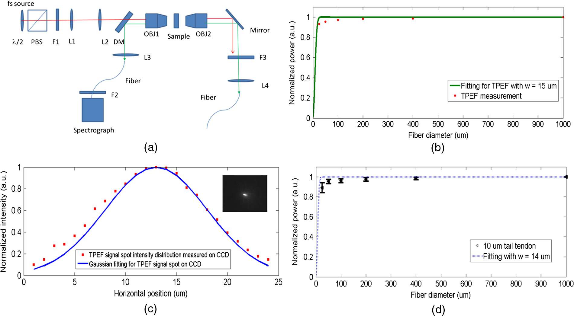$\omega =14\mu \text{m}$.

For the purpose of verifying our pinhole measurements by different core-diameter fibers, we measure the dependence of two photon excitation fluorescence (TPEF) signal on the pinhole size from a homogeneous fluorescence solution in the backward direction as shown in Fig. 3(b). Since there is negligible scattering in the homogeneous solution, only the backward generated TPEF is collected. The value of $fc/b$ equals to zero in our curve fitting because there is no scattered forward TPEF in the backward direction. It is found that $\omega =15\mu \text{m}$ provides a good fitting in Fig. 3(b). The fitting criteria follow the least square fitting such that the parameters $\omega$ and $fc/b$ minimize summation of the squares of offsets of the experimental data points from the fitting curve. The sensitivity and accuracy issue of the fitting will be discussed in the next section. The deviation from the fitting curve for a relatively small fiber diameter may be caused as the NA’s of these fibers are 0.1, while the NA’s of the rest of the fibers are 0.22. A 0.1 NA is already very close to the NA of the focusing lens L3, which is 0.11, calculated according to the focal length of L3 and the beam width of TPEF signal. In this way, the signal collection is affected slightly. Furthermore, the fiber core diameters are all large compared to the spot size under the condition of no scattering. Therefore, most of the signal is collected by the smallest fiber and the intensity change cannot be measured well by experiment. For comparison, the spot size of the TPEF signal at the focal spot of L3 is directly measured by a CCD camera (MLC 205, Matrix vision, Oppenweiler, Germany) as shown in the inset of Fig. 3(c). The $1/e^2$ spot size for the TPEF signal is $\sim 23$ and 16 μm along the horizontal and vertical directions in the CCD image plane, respectively. Figure 3(c) plots the intensity distribution along the horizontal direction on the CCD and the fitting with a Gaussian curve. Please be aware that the $\omega$ we obtained from pinhole measurement is half of the width of the signal spot size at $1/e^2$ and the full width should be 30 μm, which matches with the CCD measurement.

Similarly, we also obtain the SHG power versus fiber diameter for the 10-μm thick mouse tail tendon in Fig. 3(d). Measurements of SHG signal intensity with each fiber are repeated five times. In order to avoid significant back reflection of the forward generated SHG from the tissue/glass interface, the thin tissue samples are laid beneath a coverslip rather than being sandwiched between a coverslip and a glass slide. There is no glass slide below the sample, which is immersed in water. In 10-μm thick tissue samples, we assumed a negligible BS-SHG. Hence, the size of the focusing spot, $\omega$, can be fitted by Eq. (4) with $fc/b=0$, which is found to be 14 μm. Considering that the theoretical $1/e^2$ width of the focal spot is 0.5 μm and the theoretical magnification of the objective lens (OBJ1 $\sim 4.5\mathrm{mm}$) and focusing lens (L3 $\sim 35\mathrm{mm}$) is 7.8 times, the theoretical spot size on the CCD is estimated to be $\sim 4\mu \text{m}$. The broadening of the focusing spot in this experiment is likely due to the spherical aberration and other aberrations of lens L3, which is a spherical singlet lens.

5.

Experimental Results and Discussions

The normalized SHG signals of the mouse tail tendon tissue at three focal depths (50, 80, and 110 μm) beneath tissue surface are shown in Fig. 4(a). The sample thickness is 250 μm. Each data point represents an average of five measurements of different lateral locations at the specific focal depth. The fitted results are summarized in Table 1. Notice that when the focal depth gets deeper, the $1/e^2$ width ($\omega$ in second column) increases from 75 to 135 μm mainly due to stronger scattering of the BG-SHG. The $fc/b$ parameter (in third column) also increases with depth, consistent with MC simulations in Fig. 2(a). The ratio of BG-SHG to BS-SHG ($S_{\mathrm{B}}/c{S}_{\mathrm{F}}$ in fourth column) increases from 5.62 to 6.07. The ratio of BS-SHG to B-SHG ($\rho$ value in fifth column) decreases from 15.14 to 14.23% because, for fixed tissue thickness, the distance between focal point and rear surface of the tissue becomes smaller, which leads to less backscattering of the forward generated SHG.

Fig. 4

(a) Experiment measurement for the dependence of relative B-SHG power on fiber diameter for mouse tail tendon at different depths and the related fitting curves. (b) Contour map plotting the isolines of fitting error with various $\omega$ and $fc/b$. The sensitivities are plotted along the two dash lines crossing at the best fitting pair ($\omega =75$ and $fc/b=0.0005$) as a function of $\omega$ (c) and $fc/b$ (d). (e) The dependence of relative B-SHG power on fiber diameter for tail tendon and Achilles tendon with similar tissue thicknesses and focal point depth. (f) The dependence of relative B-SHG power on fiber diameter for Achilles tendon with different thicknesses but at the same focal point depth of 50 μm.

Table 1

A summary of the curve fitting parameters for pinhole experiment results and the derived values describing the scattering property of the tail tendon tissue at different depths.

The accuracy and sensitivity of this curve fitting method are discussed in Fig. 4(b). As we mentioned, the curve fitting is based on least square such that the parameters $\omega$ and $fc/b$ minimize summation of the square of the offsets at 25, 50, 100, 200, and 400 μm between experimental data and the fitting curve. Taking the measurements at tail tendon top as an example, summation of the offset square between experimental data and fitting curve with various $\omega$ and $fc/b$ are plotted as isolines in the contour map. The minimum sum offsets square is 0.013 (a.u.), which is from the fitting curve with $\omega =75\mu \text{m}$ and $fc/b=0.0005$. As a comparison, the sum square of the intensities at the five experimental data points is 2.56. We neglect the data for 1000 μm fiber because both experimental data and fitting curves are normalized to one at the largest fiber. Extending from the best fitting pair along the $\omega$ and $fc/b$ direction, as the two dashed lines in the contour map, the fitting errors are relatively symmetric around the best fitting parameters in Figs. 4(c) and 4(d) with similar slopes. Assuming that the F/B ratio measured for 10 μm thin samples can be approximated as the generation ratio for forward and backward SHG, i.e., $S_{\mathrm{F}}/S_{\mathrm{B}}={(\mathrm{F}/\mathrm{B})}_{\text{thin}}$, the percentage of the forward SHG that is backscattered can be calculated from the ratio of $S_{\mathrm{B}}/c{S}_{\mathrm{F}}$. The measured F/B ratio for 10 μm thin tendon is represented in the form of average (standard deviation) as 7.62 (0.81). The intensities are measured and averaged over five different positions on the tissues. Calibration of the forward and backward detection is based on the autofluorescence peak at 550 nm from the 10 μm skin tissue. The F/B absolute intensity ratio is found to be 0.5 for the fluorescence signal. All of our F/B measurements are then calibrated with this value. Some of the previous published results reveal that the F/B ratios measured for tendon are close to unity.^4,16 With the corresponding F/B ratio from thin samples, we find the proportion of BS-SHG to the forward generated SHG, which is $c={(S_{\mathrm{B}}/c{S}_{\mathrm{F}})}^{-1}/(S_{\mathrm{F}}/S_{\mathrm{B}})={(S_{\mathrm{B}}/c{S}_{\mathrm{F}})}^{-1}/{(\mathrm{F}/\mathrm{B})}_{\text{thin}}$ in Table 1 column 6. From top surface to deeper depth, $c(1)$ value varies from 2.3% (0.2%) to 2.1% (0.2%). As we have described in Figs. 2(a) to 2(c), the reduced scattering coefficient, F/B intensity ratio, and other parameters such as depth and thicknesses used in simulation are approximately the real values in experiments. Therefore, comparing the simulation with the experiment results (2.8 to 3.2% in simulation versus 2.1 to 2.3% in experiment), it is found that the simulation results are slightly greater than experimental results. This might be caused by the difference in the spot size between simulation and experiment.

We can also take the approach described in Eq. (2) to directly calculate $c$. The F/B ratio is measured at the three depths in the thick tissues directly in column 7 of Table 1. At each depth, five measurements are conducted at different lateral positions. The increase of the F/B ratio is also observed and discussed in Ref. 6 from fibrillar cellulose matrices. According to the spot size determined, the spot size in forward and backward direction should be no larger than the collection fiber core diameter of 600 and 1000 μm, respectively. Therefore, it is reasonable to assume that most of the forward and backward generated SHG are collected by our fiber collection system in their respective channels. Using the ${(\mathrm{F}/\mathrm{B})}_{\text{thin}}$ from 10 μm samples and ${(\mathrm{F}/\mathrm{B})}_{\text{thick}}$ at different depths, we obtain the parameter $c$ at different depths by applying Eq. (2), which are listed in column 8 of Table 1 indicated by $c(2)$. From top depth to deeper depth, $c$ varies from 2.4% (1.1%) to 1.6% (1.4%). These values match with the values obtained by pinhole measurements. The standard deviation of $c(2)$ is greater than that of $c(1)$ because the standard deviations of F/B ratio measurements from thin and thick tissues are transferred to the calculation of $c(2)$.

The experiment is repeated three times to calculate $\rho$ and $c(1)$ in tail tendon from three animals at different depths. The results are listed in Table 2. Note that $\rho$ and $c(1)$ are similar for the three animals. In addition, the trend such as less scattering of forward SHG with increasing depth inside the tissue is also observed among all the data sets.

Table 2

ρ and c(1) values at different depths for mouse tail tendon tissues from three animals.

In addition to comparing scattering in mouse tail tendon at different depths, we also compare the scattering in tail tendon with Achilles tendon from hind legs as shown in Fig. 4(e). The tissue thickness is 270 μm and the depth of focal point is 50 μm. The curve fitting parameters $\omega$ and $fc/b$ are obtained as 320 μm and 0.08, which provides $\rho$ as 60.9%. The F/B ratio is measured as 23 (2.5), which is close to the values measured in Ref. 7. $c$ is obtained as 6.8% (1.3%) accordingly. Compared with the results from tail tendon, at the same depth, $\rho$ and $c$ are 15.14% and 2.3% (0.2%). The $c$ value difference between tail tendon and Achilles tendon is largely due to their respective scattering coefficient difference. According to previous literature, the scattering coefficient of Achilles tendon is $\sim 45{\mathrm{cm}}^{-1}$, while that of tail tendon is from 8 to $30{\mathrm{cm}}^{-1}$.^7,15 Their F/B intensity ratios are measured to be 23 (2.5) and 7.6 (0.8). The combined effects of F/B intensity ratio and scattering coefficient determine that the BS-SHG contributes to the total backward SHG more in the Achilles tendon than in the tail tendon. In 200- to 300-μm thick tail tendon, at different depths, the BS-SHG constitutes 15% of the total backward SHG, while it constitutes $>60\%$ in the Achilles tendon. The proportion of forward SHG that backscatters is two times greater for the Achilles tendon tissue than the tail tendon tissue.

As we discussed in Figs. 2(g) and 2(h), the scattering differences are not significant when different thicknesses of tissues are compared by a relative small pinhole size. In order to demonstrate a stronger thickness-dependent BS-SHG, we replace the 35 mm focal length focusing lens L3 with another 25 mm focal length lens to reduce the beam size at the pinhole plane. Therefore, the relative collection area can be increased. The cost is that the NA of the signal can be greater than that of the collection fiber, especially for small NA fibers, which may affect the signal collection for small-diameter fibers.

In Fig. 4(f), $\rho$ and $c$ are calculated from pinhole measurements with improved collection area for Achilles tendon tissues of different thicknesses: 270, 520, and 1000 μm. The focus is fixed at 50 μm. The fitting parameters are summarized in Table 3. It is noted that $\rho$ and $c$ increase with thickness. For a 1000-μm tissue, 10.1% (1.4%) of the forward SHG are backscattered and 70.5% of the backward SHG originate from BS-SHG. This result is close to the result reported in Ref. 7.

Table 3

The curve fitting parameters and the derived ρ and c(1) values of Achilles tendon with different thicknesses at 50 μm depth.

In this study, we quantify the contribution of BS-SHG to B-SHG in two types of collagen tendon tissues with different scattering coefficients. For strong scattering tissues such as Achilles tendon, the BS-SHG dominates B-SHG. For moderate scattering tissues such as tail tendon, however, the scattering of the forward SHG is not the major source of the backward SHG. Although BG-SHG is another source of backward SHG, the mechanism for BG-SHG is still not fully understood. Conventional phase matching theory favors a forward direction in SHG generation.¹⁶ In our previous study, a similar wavelength-dependent SHG excitation spectrum was observed between the forward and backward detected SHG, which cannot be explained by the conventional phase matching theory either. These observations suggest that a nonconventional phase matching theory may be needed in order to explain the mechanism of BG-SHG in collagen tissues.

6.

Conclusions

In summary, we propose a pinhole method to investigate the scattering properties of SHG in the mouse tail tendon and Achilles tendon based on confocal multiphoton microscopy. MC simulation proves that the BG-SHG and BS-SHG can be modeled as Gaussian distribution and uniform distribution, respectively, in the pinhole detection plane. Based on the knowledge of the SHG distribution, we also obtain the spot width of the BG-SHG and the relative intensity of the BG-SHG and BS-SHG. The advantage of the pinhole method, compared with previous backscattering quantification methods, is that it is noninvasive and requires little sample preparation. Through pinhole measurements, the dependence of BS-SHG on focal depth is quantified in experiment. It is found that BS-SHG does not dominate the total backward SHG in tail tendon tissues with thicknesses of $\sim 300\mu \text{m}$. For Achilles tendon with similar thickness and focal depth, the contribution of BS-SHG to B-SHG is much higher due to its higher scattering coefficient and the F/B intensity ratio. When the thickness of the Achilles tendon increases to 1000 μm while maintaining the same focal depth, as high as $\sim 10\%$ of the total forward SHG is backscattered and collected in the pinhole. These investigations can help understand and interpret SHG measurement in microscopy and spectroscopy.