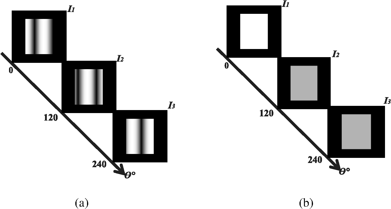
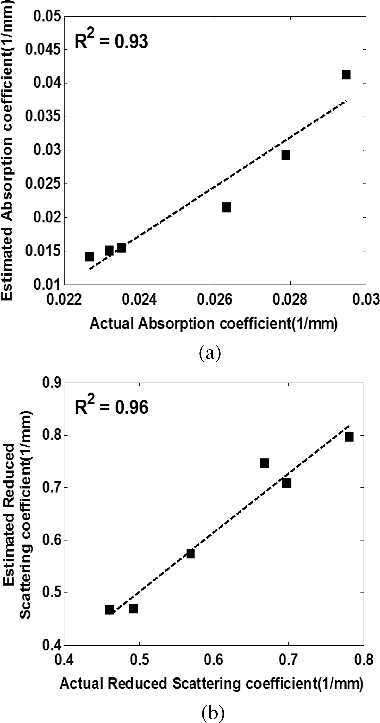
1.

Introduction

Closed head injury (CHI) is a trauma in which the brain is injured as a result of a blow to the head or a sudden, violent motion that causes the brain to move inside the skull. It is different from an open head injury in which no object penetrates through the skull. CHIs can be diffuse, meaning that they affect cells and tissues throughout the brain; or focal, meaning that the damage occurs in a local area. In both situations, CHIs can range from mild to severe and are often fatal. Common causes of CHI include blows to the head, car accidents, assault, falls, work-related accidents, sports, and serious bicycle accidents.^1–3 Typically, following injury, the level of extracellular glutamate, one of the most abundant chemical messengers in the brain, increases dramatically, causing over-stimulation of glutamate receptors contributing to neuronal cell damage and death. Excessive flow of glutamate in the brain (excitotoxic) can cause ionic imbalance and ATP depletion. Other findings include a rise in intracranial pressure, brain herniations, and vascular compressions. Eventually, these events cause changes in cell morphology as well as in hemodynamics.^4,5 Understanding neurophysiology during CHI can help the development of diagnostic strategies, optimize the treatment, and improve the therapeutic efficacy and the management of appropriate lifesaving care for head injuries. Conventional imaging modalities, such as computed axial tomography (CAT),⁶ magnetic resonance imaging (MRI),⁷ and single-photon emission computed tomography,⁸ are in common use in the evaluation of head injury. These modalities have greatly advanced our ability to understand brain function; however, each of them suffers from certain weaknesses. Moreover, the advanced hardware requirement of these techniques elevates their cost and places them beyond the reach of most bioimaging laboratories and third world countries usage. Comparatively, optical methods have garnered much attention in recent years, as they possess many advantages such as being relatively inexpensive, sensitive to several photobiological parameters, exhibiting high-spatiotemporal resolution, low risk, they are portable, and can be employed at the bedside for continuous monitoring, making them suitable for versatile biomedical applications. From a tissue optics standpoint, the physiological changes occurred during CHI can be detected by monitoring the behavior of tissue optical properties, which in turn can provide information on both hemodynamic and structural properties. The motivation for this research is to successfully detect and spatially map these properties.

The present work is part of a series of studies applying projection of near-infrared (NIR) structured illumination to study brain pathophysiology during brain injury in anesthetized rodents.^9–14 This, a relatively new large field-of-view optical imaging modality, uses a sinusoidal grid pattern to separately map tissue absorption (${\mu }_a$) and reduced light scattering (${\mu }_s^{\prime }$) properties of turbid medium such as biological samples in a noncontact and scan-free manner.¹⁵ This separation enables accurate quantification of tissue’s biochemical compositions (related to light absorption) and structural properties (related to light scattering) and thus provides a better comprehensive understanding and characterization of the corresponding tissue properties. Measurements of the changes in absorption in the NIR spectral region and the knowledge of the molar extinction coefficients of individual chromophores allow one to quantify changes in tissue chromophores such as oxyhemoglobin (${\mathrm{HbO}}_2$), deoxyhemoglobin (Hbr), total hemoglobin concentration ($\mathrm{THC}={\mathrm{HbO}}_2+\mathrm{Hbr}$), and hemoglobin oxygen saturation $[{\mathrm{StO}}_2=({\mathrm{HbO}}_2/\mathrm{THC})\times 100]$. By contrast, once the light absorption is separated from scattering effects, tissue structural properties can be studied throughout scattering properties, namely scattering amplitude ($A$) and power (sp). The advantages of this imaging technique, such as being easy to implement, relatively inexpensive (minimal number of optical elements), and scan and contact free, make it a convenient diagnostic tool to investigate the spatiotemporal changes in tissue properties under physiological and pathological conditions.

The projection of periodic illumination patterns (a.k.a. spatially modulated illumination) on a sample is not new in the area of biomedical optics, and several works have been devoted to use the same. In 1997, Neil et al. used structured illumination as a companion to confocal microscope to obtain optically sectioned images from a conventional wide-field microscope in a simple and fast operation.¹⁶ Since this report, many works have been published through the years, using structured illumination as a sectioning tool for different biomedical microscopy applications.^17–25 In 1998, Dögnitz and Wagni showed for the first time the ability of spatially modulated illumination to separately obtain the optical properties from phantoms and human skin in a noncontact manner.²⁶ A few years later in 2005, Cuccia et al. extended this technique and presented its capability to perform both diffuse optical tomography (depth sectioning) and wide-field quantitative mapping of tissue optical properties in the NIR region.²⁷ In 2011, Gioux et al. showed the first in-human study during reconstructive breast surgery in skin-flap oxygenation imaging.²⁸ As will be detailed in Secs. 2.3 to 2.5, the present study differs from previous reported structured illumination methods ^9–14,27,28 in the simplicity in the way the optical properties were obtained (using high- and low-spatial frequencies) and in the calibration procedure. Out of these, for the reader’s knowledge, the use of sinusoidal pattern is also popular as a super-resolution platform,²⁹ in machine vision,³⁰ and in the area of optical image processing, specifically when three-dimensional (3-D) object surfaces measuring (profilometery) is on-demand.^31–36 As far as we aware, 3-D surface measurements are used as a diagnostic tool in biology and medicine societies in dentistry,^37,38 cardiology,³⁹ endoscopic,⁴⁰ and orthopedics.⁴¹

Taking advantage of the aforementioned technique, this article’s main focus is the application of structured illumination to study brain hemodynamic and morphologic changes following CHI in intact rodent heads. In addition, to the best of our knowledge, the literature on using optical modalities and specifically optical-imaging techniques to study CHI is scant. There is little existing literature on CHI effects on brain tissue optical properties. Recent work using diffuse correlation and reflectance spectroscopy during diffuse axonal injury (type of CHI) was used in neonatal piglets ($n=18$) to monitor cerebral blood flow (CBF) and hemodynamic parameters before injury and up to 6 h after the injury.⁴² Recently, we quantitatively studied brain hemodynamic and morphological variations during CHI in intact mice heads ($n=16$) for the first 60 min using orthogonal diffuse NIR reflectance spectroscopy.⁴³ Mapping brain optical and physiological properties following CHI is the main difference separating the present research from the above studies. This gives us the ability to simultaneously monitor different brain regions and to explore and compare those areas in response to injury at high-spatial resolution, a merit that is not available when a single optical fiber (point image) is used. As far as we aware, this is the first demonstration of implementing this technique through the intact scalp to evaluate the pathophysiological state of the brain in response to CHI.

The rest of the work is organized as follows: Sec. 2 outlines the essential details of our animal model, system operation, physiological quantification analysis, and calibration procedure. Section 3 shows experimental results and discusses issues related to these results. Finally, Sec. 4 summarizes the work.

2.

Materials and Methods

2.2.

Instrumentation

The schematic layout of the imaging setup is illustrated in Fig. 1 and is identical to that described in detail elsewhere.⁹ In short, sinusoidal patterns illuminate the head three times at the same spatial frequency $f_x$ (one-dimensional pattern) with a phase difference of 120 deg,

Eq. (1)

$$S_i(x,y)=\frac{S_0}{2}[1+m\cos (2\pi f_x+{\varphi }_i)],$$

where $S_0$ is the illumination source intensity, ($x,y$) denote the coordinate axes, $m$ represents the modulation contrast, and ${\varphi }_i$ is the spatial phase (${\varphi }_1=0$, ${\varphi }_2=120\mathrm{deg}$, and ${\varphi }_3=240\mathrm{deg}$). Patterns, which can be programmed as simple slideshows on a personal computer, are serially projected via modified commercial multimedia projector (PLUS, U5-112, $800\times 600\text{pixels}$) using digital light processing (DLP) that created the sinusoidal pattern and was controlled by a personal computer (Intel E8500). The original lens system of the projector was changed in order to adjust the field of illumination to a size of millimeters (instead of meters). Additionally, the color filter inside the projector was removed so that the projected patterns are actually all in the grayscale mode. These patterns are then passed through an automatic six-position filter wheel (Thorlabs, New Jersey, FW102C) placed immediately at the output of the projector. The filters were 10-nm bandpass filters centered at wavelengths of 650, 700, 720, 800, 880, and 920 nm (Thorlabs, FB Series). The diffusely reflected light, which encodes brain tissue optical properties information, is imaged with an 14-bit CCD camera (Prosilica, Stadtroda, Germany, GX1920) with a pixel size of 4.5 μm mounted normal to the brain surface interfaced to a personal computer. The camera, equipped with an imaging objective lens (Kowa $f/2.8$, Japan), is capable of imaging up to 40 frames per second at full $1936(\mathrm{H})\times 1456(\mathrm{V})$ resolution covering the wavelength region of 400 to 1000 nm. The mirror appearing in the setup directed the projected pattern onto the head and was aligned at a small angle of incidence to the normal direction to avoid the detection of specular reflected light. It is worth pointing out that, within this system, the temporal resolution is determined by the time required to project the patterns, the color wheel rotation, and the acquisition time of the camera. In contrast, spatial resolution depends mainly on the CCD camera, illumination spatial frequency, system noise, and the medium optical properties.¹⁵

Fig. 1

Schematic representation of the near-infrared (NIR) structured illumination instrument, showing the major components and the pattern paths.

2.4.

Physiological Properties Quantification

In contrast to the traditional spatial frequency domain–imaging data analysis described in Ref. 15, here we use a different approach to quantify absorption and reduced scattering coefficients of the mouse brain. It has already been shown that at higher spatial frequency, we are strongly sensitive to scattering changes, whereas low-spatial frequency has most sensitivity to changes in absorption.⁴⁶ High-spatial frequency is analogue to small source-detector separation (SDS), in which the detected reflected light is dominated by shorter path length photons (short depth). On the contrary, large SDS is equivalent to low-spatial frequency, in which the detected reflected light is dominated by longer path length photons (longer depth). For this reason, measurements at two spatial frequencies, low and high, can result in different sensitivities to absorption and scattering, which in turn enable one to quantify separately the optical properties of a sample under investigation. We therefore employ only two modes of spatial frequency (low and high) in our instrument. With high-spatial frequency, the reduced scattering coefficient at each wavelength was approximated as follows:

Eq. (2)

$${\mu }_s^{\prime }(\lambda ){|}_{f_x>0}\propto \sqrt{{(I_1-I_2)}^2+{(I_1-I_3)}^2+{(I_2-I_3)}^2},$$

where $I_1$, $I_2$, and $I_3$ represent the reflectance images with spatial phases of 0, 120, and 240 deg, respectively, at the same spatial frequency. A demonstration of $I_1$, $I_2$, and $I_3$ projected onto the head is shown in Fig. 2(a). By using Eq. (2), we have the ability to map the scattering properties at each wavelength on a pixel level. Averaging over each ${\mu }_s^{\prime }$ image area at each wavelength ($\lambda$), the scattering spectra of brain tissue can be derived, and the scattering power–law relationship^47–49 is fit to obtain scattering properties ($A$, sp) as follows:

Eq. (3)

$${\mu }_s^{\prime }(\lambda )=A{\lambda }^{-\mathrm{sp}}\mathrm{.}$$

Fig. 2

Example of projected structured pattern at $f_x>0$ (a) and $f_x=0$ (b).

By analyzing the spectra of scattered light, information regarding the morphology and composition of cells can be retrieved: specifically, $A$ is the scattering amplitude presumed to be related to the density of the scatterers (cell membrane, organelle membrane, cell nuclei, and other intracellular organelles including the mitochondria), their distribution, and refractive index changes, and sp (wavelength exponent) is the scattering power typically dependent on the mean size of the tissue scattering particles and it defines spectral behavior of the reduced scattering coefficient.⁵⁰ A small value of sp corresponds to larger scatterers’ size, while the higher values correspond to smaller scatterers’ size. Together, $A$ and sp reflect changes in structural composition.

Phase shift is meaningless at low-spatial frequency ($f_x=0$), as shown in Fig. 2(b). Therefore, the absorption coefficient was approximated by the following expression:

Eq. (4)

$${\mu }_a(\lambda ){|}_{f_x=0}=\frac{1}{3}(I_1+I_2+I_3)\approx I_1\mathrm{.}$$

Although low-spatial frequency is more sensitive to absorption changes, in order to reduce the influence of scattering, Eq. (4) was modified accordingly by subtracting the scattering

Eq. (5)

$${\tilde{\mu }}_a(\lambda )=\mathrm{Eq.}(4)-\mathrm{Eq.}(2)$$

Note, before subtraction images were normalized and absolute operation was made to prevent negative absorption values. Furthermore, with measurement of absorption at each wavelength combined with the wavelength-dependent molar extinction coefficients $[\epsilon (\lambda )]$, the absolute concentration of individual chromophores can be deduced (Beer’s law^51,52)

Eq. (6)

$$\overrightarrow{c}={({[\epsilon (\lambda )]}^T[\epsilon (\lambda )])}^{-1}{[\epsilon (\lambda )]}^T{\overrightarrow{\tilde{\mu }}}_a·\overrightarrow{k},$$

where $\overrightarrow{c}$ is the chromophore molar concentrations vector of length $M$, ${\overrightarrow{\mu }}_a$ is the calculated absorption coefficients from Eq. (4) of length $N$, $[\epsilon ]$ is the known molar extinction coefficients matrix for each chromophore^53–55 with size $N\times M$, $\overrightarrow{k}$ is the proportionality coefficient vector of length $M$, and the upper letter $T$ represents transpose matrix. Routinely, constrains that are usually employed is a positive value of concentration; negative values are not allowed. Since in mice the layers are optically thin ($\text{skull}=500\mu \text{m}$, $\text{brain}=1\mathrm{cm}$, etc.), the provided values of both optical properties and chromophores in this article will be consider as an average value resulting from sampling a single volume (homogenous medium). The above properties steps are summarized in the block diagram shown in Fig. 3.

Fig. 3

Flow chart describing the process of getting the physiological parameters with two spatial frequencies.

2.5.

Calibration Strategy

A calibration procedure was utilized to: (1) reduce errors in the measurement of optical properties as a result of the approximation made in Eqs. (2) and (4); (2) overcome nonlinearity in camera exposure time at different wavelength used; (3) other system variability’s such as source fluctuations and DLP nonlinearity. The calibration involves the use of a tissue-like phantom as a reference with known optical properties over the wavelength range 600 to 1000 nm to determine scale factors, $K_s(\lambda )$, $K_a(\lambda )$, as estimators for the true values of scattering and absorption coefficients, respectively. These factors will be used later to multiply Eqs. (2) and (4) for future validation of unknown optical properties. After $K_s(\lambda )$ and $K_a(\lambda )$ were determined, a new phantom with known optical properties was measured, and the estimation of the same was obtained and compared with the true values (validation process). Correlation between the actual (reference) value of optical property and measured (estimated) value was evaluated and is plotted in Fig. 4 for absorption [Fig. 4(a)] and scattering [Fig. 4(b)], respectively. As can be seen in Fig. 4, the estimated values are in good agreement with the original values, reflected by high correlation between the two, and demonstrate good use of the scale factors for estimating absorption and reduced scattering coefficients. The above calibration procedure was performed right before and after each of the experiments to achieve accurate measurement of the optical properties and to determine system reliability and robustness. On the basis of the aforementioned procedure, the absorption and scattering coefficients in the brain were derived using the coefficients obtained from the calibration.

Fig. 4

Estimated against actual values for absorption (a) and reduced scattering (b) coefficients during validation process in tissue phantom experiments. The broken line is the best-fit linear regression fits to the data (squares). High correlation was obtained with $R^2=0.93$ and 0.96, respectively.

3.

Results and Discussion

Figure 5(a) is a typical photograph of a shaved animal head captured on a CCD camera from a representative mouse. The dotted-line box denotes the ROI selected by the investigators for analysis. The location where the weight dropped is also shown in the figure. Figures 5(b) and 5(c) show the ROI with two spatial frequencies of $0{\mathrm{mm}}^{-1}$ (DC frequency) and $0.16\text{lines}/\mathrm{mm}$ (AC frequency) at 650 nm, respectively. Each image in Figs. 5(b) and 5(c) covers an area of $\sim 3\times 3{\mathrm{mm}}^2$, which corresponds to $200\times 200\text{pixels}$, and results in spatial resolution of $0.015\mathrm{mm}/\text{pixel}$. As noted in the previous section, light scattering can provide valuable information on tissue structural properties’ changes such as density, size, and distribution of scatterer. Hence, examination of the dynamic scattering behavior can indirectly provide fundamental insight into microstructural features. With that, maps and the corresponding pixel histogram distributions of the resulting reduced scattering coefficient, for demonstration at 650-nm pre- and 10-min post-CHI, were generated from the set of three images as based on Eq. (2) and are shown in Fig. 6. The mean reduced scattering $\text{coefficient}\pm \text{standard error}$ given above each image was obtained using mean2 and std2 functions in MATLAB over each image. The grayscale in the right side of each map panel represents the absolute scattering value of each pixel in the image. Higher scattering values correspond to brighter pixels and vice versa. In the figure, an 11% reduction in scattering 10-min after CHI is recovered. With this, a dynamic time course of the scattering within the entire ROI pre- and post-CHI is plotted in Fig. 7, respectively. As can be seen, stability in measurements over time is obtained, and scattering contrast after injury is shown with an overall 12% reduction in scattering accompanied by a small error deviation. Stability indicates that there was no influence of possible artifacts during measurements. The reduction in scattering may be attributed to several cellular morphological changes, such as swelling, pyknosis, chromatolysisetc, etc., in response to injury and subcellular responses (organelle changes) that reduce the optical density of the brain tissue as well as change the refractive indices (sample inhomogenity). These results are in a good agreement obtained by our previous report following CHI⁴³ and ischemic stroke.⁹

Fig. 5

(a) Wide-field reflectance image of the animal head as captured by the CCD camera. The dotted line box is the region-of-interest (ROI) selected later by the investigators for processing. ROI (b) when $f_x=0{\mathrm{mm}}^{-1}$ (DC frequency) and (c) when $f_x=0.16{\mathrm{mm}}^{-1}$ (AC frequency) at different phase shift. ROI size equals to $\sim 3\times 3{\mathrm{mm}}^2$ ($200\times 200\text{pixels}$). In all panels, a 650-nm illumination was used for demonstration purpose.

Fig. 6

Reduced scattering coefficient map and pixel histograms of pre- (a) and (b) 10-min post- closed head injury (CHI) at 650 nm. A bar showed the value of scattering in each map. Histograms indicate the degree of spatial variation in recovered reduced scattering coefficient. The grayscale in the right side of each map panel represents the absolute scattering value of each pixel in the image.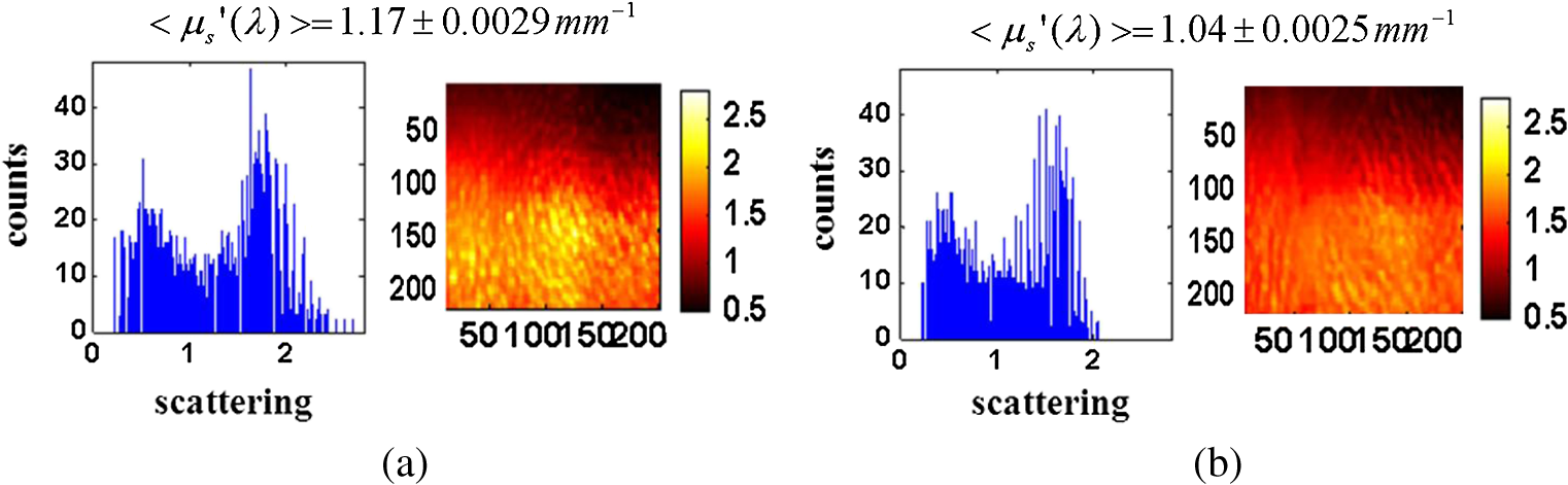

Fig. 7

Time traces of the reduced scattering coefficient of brain tissue pre- (a) and post-CHI (b) at 650 nm. Dotted line represents the average. Cell volume changes as well as changes in the distribution and structure of organelles cause changes in light scattering.

As mentioned in Sec. 2.4, by the knowledge of the scattering at each wavelength, the scattering spectra can be derived overtime as presented by the plots in Fig. 8 for three representative time points. Not seen in the graphs are the (small) error bars of the standard error. Fitting scattering values based on Eq. (3) resulted in the power–law expression with the scattering amplitude ($A$) and power (sp) as appears in each graph; the points represent the discrete calculated reduced scattering coefficient at specific wavelengths, and the dashed line represents the power-law fit to this data. Cleary observed the decrease in both $A$ and sp, which reflects the structural changes following CHI. Because of its high values, the logarithmic value of $A$ was taken. To highlight the change in sp and hence the variation in the slope during the fitting procedure, we present in Fig. 8(d) the normalized scattering spectra of Figs. 8(a)–8(c); sp decreased by 28% and 54% in 10 and 45 min, respectively, from baseline. That is, as we move from baseline to injury state, the scattering slope becomes progressively flat, reflecting the increase in particle size or the evolution of swelling of the cells and cell organelles in the brain due to ion and water movements, membrane breakdown, and capillary changes. As stated above, this behavior demonstrates the morphologic changes that occurred in the brain during CHI and highlights the presence of cellular swelling within brain parenchyma.^{10,43,56–58}

Fig. 8

Reduced scattering spectra in preinjury (a), 10-min (b) and 45-min post-CHI (c). The points represent the calculated reduced scattering coefficient at specific wavelengths, and the dashed line follows the power–law fit to this data. Standard errors are hardly shown in all these graphs because of low-error level. Discrepancies in equations are clearly observed and represent brain structural changes. (d) Normalized reduced scattering spectra following CHI at the above three representative time points. The change in the scattering slope potentially emphasizes the evolution of brain edema (increased astrocytic swelling) and decrease cellularity following injury. These results were reproducible for the other four mice examined.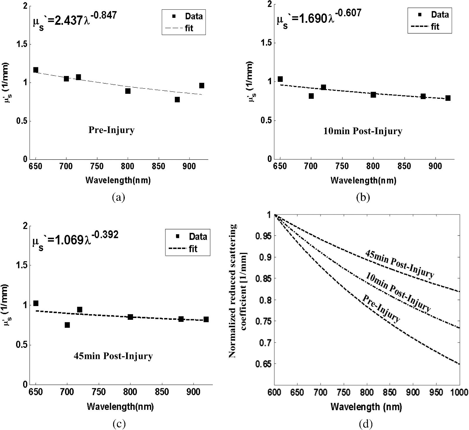

For completeness of scattering processing, we next present qualitative image maps of both $A$ and sp. At this point, we have a spectral cube with dimensions of $200\times 200\times 6$, where $200\times 200$ is the 2-D image pixel size and 6 stands for the number of the wavelengths used. By scanning individual columns of the cube and fitting the data with Eq. (3), two matrices are concomitantly built: one for $A$ and the other for sp, where each pixel in each matrix corresponds to the calculated $A$ and sp, respectively. As a continuation of the previous figure, qualitative image maps at the above same three time points are displayed in Fig. 9. The grayscale in the right side of each map panel represents the scattering property value of each pixel in the image. Besides each map, we display the histogram distribution of the corresponding ROI. By converting $A$ and sp maps into histogram distributions during CHI, an additional insight of the regional changes of the brain on a pixel level can be obtained. As seen, sp decreases following CHI as reflected in brighter pixels in the map, while the decreases in $A$ are reflected in more dark pixels. Averaging these maps reveals the following results: (1) 10-min post-injury, the sp decrease by 35% and by 58% after 45 min from baseline and (2) there is a decrease of 38% and 63%, respectively, in $A$ for the same time points.

Fig. 9

Maps and pixel histograms of the scattering power (top) and amplitude (bottom) preinjury (a), (b) 10-min, and (c) 45-min post-CHI. The average change following CHI are clearly demonstrated in comparison to the baseline (a). These qualitative image maps give an additional insight (spatial and temporal) of the regional structural changes of the brain on a pixel resolution level.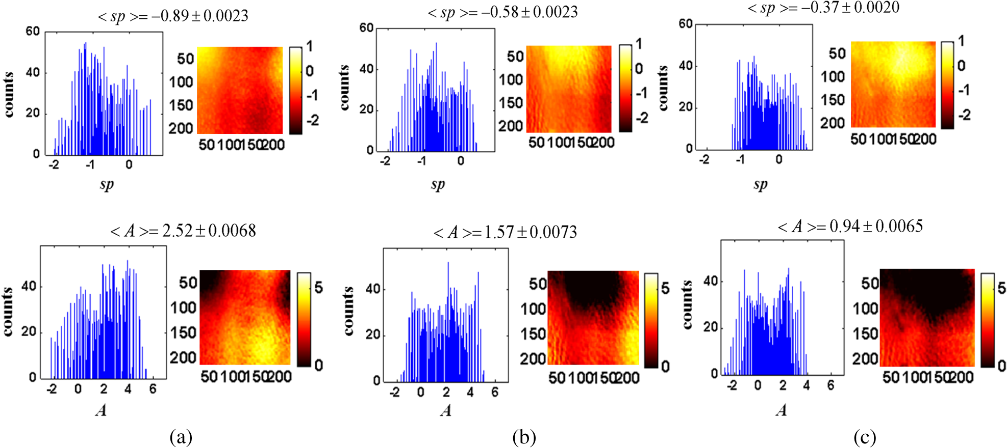

Finally, Fig. 10 gives the dynamic time course of sp and $A$ pre- and post-CHI. We assume that the decrease in $A$ reflects the change in the ratio of the refractive index outside (extracellular) to inside (intracellular) the scattering particle. This reduction in spatial variation of refractive index causes more light to pass through the brain and less light to be scattered, which also explains the observed reduction in scattering coefficient (Fig. 7). Reports of monitoring light scattering during brain injury are limited or have not been presented before. The above figures of scattering properties demonstrate our ability to provide complete information and more insight on cerebral tissue spatial structural variations and properties following CHI on a pixel basis, which is a primary advantage of this technique in comparison to other optical modalities such as optical coherence tomography⁵⁹ or photo-acoustic tomography.⁶⁰ In addition, these results show a very good sensitivity of structured illumination to detect spatial variation in reduced scattering coefficient or alternatively morphological changes.

Fig. 10

Time courses of the scattering power and amplitude in pre- (a) and post- (b) CHI. This trend in $A$ and sp was reproducible for all mice examined. Dotted line represents the average. Note that we decide to report the logarithm of the scattering amplitude ($A$), since the range of $A$ was quite large due to some extreme values. In all these panels, the coefficient of variation for repeated measurements of cerebral optical scattering properties was $<5\%$. These results were reproducible for the other four mice investigated.

Optical scattering describes the probability of light being deflected by the structural components of tissues, while optical absorption represents the process of light attenuation by chemical components within the sample. Therefore, by calculating the absorption coefficient at different wavelengths [Eq. (5)] and the knowledge of the wavelength-dependent molar extinction values of tissue chromophores enables us to obtain tissue composition concentration via the Beer’s law [Eq. (6)]. Figure 11 demonstrates that the resulting absorption coefficient map and its corresponding histogram distributions are recovered at 650 nm pre- and 10-min post-CHI. Above the map and the histogram is the mean absorption ± standard error obtained by calculating the same over the image map. In addition, the averaged absorption coefficient versus wavelength over the spectral range 650 to 920 nm is given (absorption spectroscopy). Clearly observed changes in absorption values in these two panels highlight the changes in brain tissue composition and the abilities of NIR structured light technique to detect and map absorption variations over time. As mentioned, by mapping the absorption coefficient at each wavelength and the knowledge of the extinction molar coefficients, a quantitative hemodynamic concentrations map of each chromophore can be obtained. Averaging each individual map over time, the time traces of chromophores before and following CHI were achieved as is shown in Fig. 12. The effects of injury on tissue chromophore are clearly visible in the graphs; as we progress from normal state (baseline) to injury state, an increase in deoxyhemoglobin (Hbr) by 30% was found and may relate to increased capillary and venous blood stases during injury coupled with a decrease in oxyhemoglobin (${\mathrm{HbO}}_2$), THC, hemoglobin oxygen saturation (${\mathrm{StO}}_2$), and lipids from baseline measurements by 45%, 11%, 22%, and 4%, respectively. It can be seen that after CHI, the ${\mathrm{StO}}_2$ level (usually between 60% to 70%) dropped by more than 20% and then starts gradually to increase toward baseline level. A drop in ${\mathrm{StO}}_2$ indicates decreased oxygen delivery to the brain and energy failure that can lead to permanent brain damage, neurological disorders, or even death. Similar findings on ${\mathrm{StO}}_2$ behavior after injury (slow decrease) were also observed by Yodh’s group during axonal injury in piglet brains (Ref. 42, Table 2, p. 5411). In a different model of cerebral hypoxic-ischemic insults in piglets reported by Ioroi et al., a similar recovery in ${\mathrm{StO}}_2$ within a few minutes as that observed here was demonstrated.⁶¹ The decrease in ${\mathrm{StO}}_2$ level we observed reflects the acute effects of neurotrauma and the brain’s response during the early minutes of injury. Assuming constant hematocrit level, THC can serve as an indicator to cerebral blood volume variations and hence to CBF; CBF is one of the most important determinants of brain oxygen delivery. We hypothesize that the fluctuations in CBF level may represent the well-known mechanism of cerebral autoregulation (CAR), in which the brain tries to maintain a constant blood flow by constantly changing cerebral vascular resistance in response to changing arterial blood pressure or cerebral perfusion pressure. In order to pursue further this hypothesis, laser Doppler as well as systemic blood pressure measurements will be used in our ongoing research. Generally speaking, disturbed CAR can reduce the ability of injured brain to preserve an adequate blood flow as clinically observed in patients with mild and severe brain injuries.^62–64 Because THC decreases as a result of the injury, a decrease in local arterial blood may concurrently occur, likely due to a combination of intracranial hemorrhage and cerebral contusion (bruising of brain tissue). Moreover, focal injury, such as CHI, is characterized by reduced CBF which leads to disruption of oxygen balance (supply versus demand) and results in metabolic changes in the injured area. Reduction in CBF is consistent with previous data reporting the alteration in CBF following traumatic brain injury on both human and animal models.^65,66 In the model presented here, were 50 g weight dropped from a height of 90 cm, bruising, torn tissues, bleeding and other physical damage to the brain can be presented. These global physiologic changes can result in long-term complications or death as we observed during some experiments. For this particular study, since it was out of the scope of our study, we did not perform histological observations on the status of hemorrhage and/or contusion in the brain; however, no blood breakdown products were observed in the scalp during the experiments. Future studies are warranted to determine the status of the brain following this model of injury. In addition to the hemodynamic changes of the above representative mouse, measurements of the systemic physiological parameters over time were monitored and showed a decrease in both ${\mathrm{SpO}}_2$ ($89.52\pm 2.27\%\to 66.41\pm 1.73\%$) and HR ($134.5\pm 11.32\mathrm{rpm}\to 122.3\pm 2.89\mathrm{rpm}$) which reveals a decrease of $\sim 25\%$ and $\sim 10\%$, respectively, from the baseline. We also calculate these systematic parameters from the entire study and found a decrease of $\sim 28\%$ in ${\mathrm{SpO}}_2$ ($89.43\pm 1.8\%\to 64.16\pm 3.7\%$) and decrease of $\sim 15\%$ in HR ($167.07\pm 8.3\%\to 142.45\pm 4.1\%$). The lack of oxygen, which affects the function of the cellular respiratory activity, reflects the severity of the injury model used and probably that the damage reached the brainstem.

Fig. 11

Map and pixel histogram of the absorption pre- (a) and (b) 10-min post-CHI at $\lambda =650\mathrm{nm}$. The average value of the absorption coefficient is given. The grayscale in the right side of each map panel represents the absolute absorption value of each pixel in the image. Below the map and histogram is the absorption spectrum for each time point. The point represents the calculated absorption coefficient at specific wavelengths, and the dashed line represents the spline interpolation to this data.

Fig. 12

Typical time series of brain absolute hemodynamic value pre- (left) and following CHI (right). The average value is given above each individual chromophore. Our ability to quantify changes in chromophore concentrations over time is clearly demonstrated. In all the above panels, the coefficient of variation for repeated measurements of cerebral hemodynamics was $<6\%$. Similar trend of the hemodynamic response was observed across the other mouse experiments.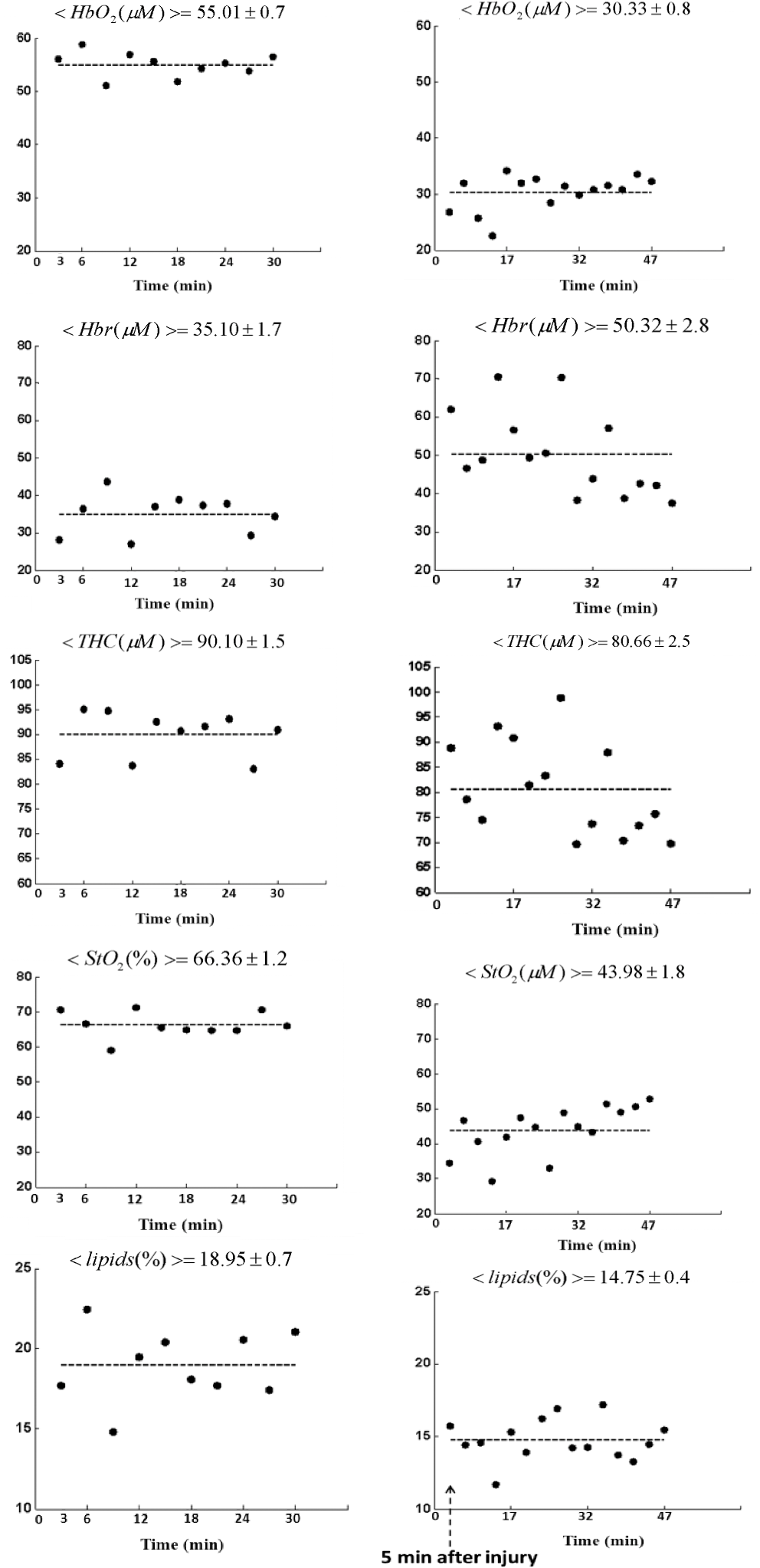

These overall hemodynamic changes throughout the injury period delineate: (1) the pathophysiologic state of the brain in response to CHI, (2) changes in brain hemodynamics, (3) agree reasonably well with the results available in the literature,^67–74 and (4) reflect our ability to follow brain physiological properties over time during injury. In contrast to ${\mathrm{HbO}}_2$, Hbr, THC, and ${\mathrm{StO}}_2$, tissue lipid levels did not change substantially during injury within this representative mouse, $\sim 4\%$ from baseline. This result stands well with the entire study result as can be seen in Fig. 15. In general, variation in lipid may be an indication of the dysregulation of lipid metabolism within brain cells.^75,76 Altered lipid metabolism is believed to contribute to secondary brain injury, which occurs after traumatic brain injury. Nonetheless, our findings of alterations of lipid during CHI are preliminary and will be pursued in a future work. Unfortunately, water concentration is not presented in this study due to the low-quantum efficiency ($\sim 5\%$) of our CCD camera around 970 nm that results in poor signal-to-noise ratio. It is true that water is a dominant chromophore that has several features at a few NIR wavelengths (760 and 830 nm) and can be included during Beer-Lambert fitting; however, the extraction of an accurate water value in those wavelengths (small values in comparison with ${\mathrm{HbO}}_2$ and Hbr) required more advanced mathematics/broadband fitting techniques,^77–80 which are beyond the scope of this work. It is important to mention here the point of water fitting: since the absorption coefficient of water is temperature dependent, the fitting process needs to be adapted continuously in order to account for possible temperature effects, which complicates the fitting process. In the current study, the information on water changes was deduced indirectly through the sp parameter as discussed above. Our previous research on CHI using diffuse spectroscopy reveals an average change of 6% in water concentration following acute CHI as a result of brain edema evolution.⁴³ In the future, we plan to study water variation following CHI with an adequate high-quantum efficiency camera. In comparison to Ref. 43, a slight difference in the behavior of ${\mathrm{HbO}}_2$, and in THC as consequence, was observed. Several reasons could explain these differences, among which we can cite: first, the small measurement volume of a single-point fiber probe used in that study can lead to spatial variability of tissue property values. Second, a different algorithm which was used here for absorption evaluation (diffuse reflectance light is subtracted from scattering) may be a possible explanation for the difference. Third, we acknowledge that with imaging, a large area (injured and noninjured regions) is sampled and therefore regional heterogeneity of brain tissue and volume effect (sampling different layers) can highly influence the measured absorption values. Fourth, there will always be some slight variability in the impact energy delivered from mouse to mouse and in the physiologic response of each animal. Fifth, with the relatively small numbers used, there might be slight variations in experimental results. Despite these, it is clear that simultaneous experiments with both setups (diffuse spectroscopy and NIR structured illumination) and similar data processing should be further investigated with greater numbers of animals for better understanding the difference and for more conclusive and unequivocal results.

A typical series of structured illumination chromophore maps delineate the dynamic spatial and temporal changes over the ROI at three representative time points, 0, 10, and 45 min following CHI, is shown in Fig. 13. For better visualization and presentation, we show the map of each chromophore after using Savitzky-Golay differentiation filtering and normalization. Low concentration values correspond to lower pixel reflection as more dark pixels and vice versa at high concentration values, as represented by the scale bar to the right of each map. Although the absolute chromophore value of each pixel is in an arbitrary unit, the effects of injury are clearly visible, highlighting the trend in chromophores and our distinguishability following injury.

Fig. 13

Series of the spatiotemporal chromophores map distribution following CHI at three different representative time points. Scale is normalized, and maps were filtered for better visualization. During the progress of injury, structured illumination is able to map and follow difference in intact brain hemodynamic over time.

Lastly, we explore the variation in the ratio between the scattering to absorption (${\mu }_s^{\prime }/{\mu }_a$) and in the transport albedo coefficient ($a^{\prime }={\mu }_s^{\prime }/{\mu }_a+{\mu }_s^{\prime }$) as a function of wavelength pre- and post-CHI from the above representative mouse, as depicted in Figs. 14(a) and 14(b), respectively. From Fig. 14(a), we can see a high ratio, ranging from 20 to 90, which confirms the known fact that brain tissues are highly scattering media.^81–84 In addition, this high ratio justifies the use of diffusion approximation (not used here) to model photon transport in brain tissue.^85–88 Linear regression was used to compare the change in slope of the regression. As seen, when we move from baseline to injury state, the slope decreases progressively by more than 10%, probably a reflection of cellular/vascular responses to the injury. In all graphs, high correlation was achieved ($r>0.97$) and significance ($p<0.001$) of the slope over time was found, highlighting the possibile use of the same as an additional marker for injury status. In Fig. 14(b), the albedo graph shows a high value ($a^{\prime }\ge 0.97$) over time. Although Fig. 14(b) repeats in principle the results from Fig. 14(a), the stability in $a^{\prime }$ in comparison with the changes observed in the ratio ${\mu }_s^{\prime }/{\mu }_a$ cannot reveal changes in the optical properties but can only indicate the characteristics of the medium under test (low absorption and high scattering), which is important sometimes where there is an attempt to use different light modeling approximations.^89,90

Fig. 14

(a) The ratio between reduced scattering coefficient to absorption coefficient in the range 650 to 920 nm at the baseline (top), 10-min (middle), and 45-min (bottom) post-CHI, which demonstrates monotonic decrease with wavelength. A linear relationship with excellent correlation ($r>0.97$) and varying slope were obtained (confidence interval $\sim 7\%$). The fitting line is represented (broken line). As we move from baseline to injury state, the slope decreases progressively by more than 10% for this representative mouse. (b) Transport albedo coefficient in the range 650 to 920nm at the baseline (top), 10-min (middle), and 45-min (bottom) post-CHI. By opposition, the albedo coefficient remains about the same as we move from baseline to injury state.

We repeated the above experiment and analysis in a series of another four injured mice with similar body weights and type using the same setup and model. Figure 15 summarizes the statistical analysis of the average injury effect on chromophore concentrations and scattering properties made in the study over the same ROI at four different time points after CHI. Compared with preinjury values, CHI was found to have a significant impact on ${\mathrm{HbO}}_2$ and ${\mathrm{StO}}_2$ following injury: ${\mathrm{HbO}}_2$ dropped gradually to a very low level during the whole injury period, while ${\mathrm{StO}}_2$ increases slightly after 20 min, but then further decreases, probably because of a decrease in oxygen delivery to the brain and a decrease in blood supply to the injured zone. Generally speaking, cerebral oxygen delivery is dependent upon the cerebral perfusion pressure and the oxygen content of blood, which is principally determined by hemoglobin. As seen, significant changes were also found in Hbr by 10- and 30-min post-injury. In all other parameters, a decrease from baseline level is seen with no statistical significance. It was somewhat surprising to us that with this severe model, significance was not presented in the scattering power (sp), which reflects brain cells swelling or edema evolution. Nonetheless, a change of up to 10% in sp from baseline over time was observed. Since cells’ swelling or edema can occur sometimes over a period of hours or days, we believe that monitoring over a long period of time will increase sp significance. In all presented parameters, no return to baseline level was observed, which emphasizes the severe condition of the brain and its lack of ability for self-recovery over time. It should be pointed out that CHI can create zones of damage: a core area with severe damage and surrounded area suffers moderate damage. Because both areas are simultaneously imaged within our system, it may affect the obtained results. This may be a possible explanation of the difference in behavior between chromophores and structural changes and the fact that tissues with different degrees of injury will have different oxygenation states.

Fig. 15

Bar graph summarizes hemodynamic and morphologic parameters for different time points. The results are presented as a $\text{mean}\pm \mathrm{SE}$ ($n=5$). Significance of the difference between pre- to post-injuries are marked with asterisks: *$p<0.05$, **$p<0.01$, and ***$p<0.001$. Note: $A$ and sp were scaled to fit the $y$-axis by 100 and 10, respectively.

As is evident from the results, the pathophysiology of brain injury is very complicated and not fully understood. The cascade of events that occur following brain injury involve a subtle interplay between CBF, oxygen delivery and utilization, and supply of main cerebral energy substrates (glucose) to the injured brain. Regulation of this interplay depends on the type of injury and may vary individually and over time.^91,92 In the early phase following brain injury, a complex series of pathologic events triggers the propagation of a secondary injury cascade to cerebral areas initially not involved by brain injury. These include inflammation, oxidative stress, ionic imbalance, increases in vascular permeability, mitochondrial dysfunction, etc.⁹³ Considering that capillary architecture has a central role in oxygen delivery to the cell, changes in red blood cell transit time through capillaries could indicate hypoxia in the injured brain, despite a normal blood volume. Supporting the injured brain with adequate CBF and delivery of oxygen and energy substrates, therefore, are a mainstay of therapy after brain injury. Microvascular damage following brain injury accounts for the inability of pericontusional tissue to increase the oxygen extraction fraction (OEF—fractional conversion of oxygen from arterioles to venules) in response to the reduction of CBF induced by hyperventilation. Brain activation and any augmentation of energy demand are followed by an increase in CBF and OEF.⁹⁴ Glucose utilization may increase dramatically after brain injury in the absence of oxygen or CBF limitation (cerebral hyperglycolysis). This may lead to a reduction of cerebral glucose below the critical level and to a state of brain energy dysfunction or crisis.⁹⁵ In addition, cerebral oxidative metabolism may also be impaired due to mitochondrial dysfunction, and thereby result in reduction of cerebral metabolic rate of oxygen (${\mathrm{CMRO}}_2$) in the acute period after brain injury.

In summary, the changes we observed in this work reflect the pathophysiologic state of the brain following CHI (damaged blood vessels, extravasation of blood, vasospasm, increased neuronal cell death, etc.) and confirm the potential use of structured illumination as a medical tool to quantify changes in chromophore concentrations and morphologic variations in an intact brain over time during CHI.

4.

Conclusion

Normal brain function depends on delivery of oxygen, glucose, nutrients and on clearance of the byproducts of metabolism. During CHI, these mechanisms are altered, leading to neuronal damage. Specifically, following injury, reduction in CBF causes a disruption in oxygen balance, leading to interruption of extracellular ion balance, an increase in lactate levels, a decrease in extracellular pH, abnormal accumulation of glutamate, etc.⁹⁵ Understanding the complex physiological state of the brain following injury would greatly help in the development of diagnostic or therapeutic strategies. To this end, we hypothesize that optical imaging-based NIR structured illumination can be utilized to study cerebral hemodynamic and structural parameters’ responses to CHI challenge. In the present study, we investigate and demonstrate the feasibility of using the same as a monitoring tool for concurrently tracing and mapping brain pathophysiologic parameters in an intact mouse head during injury. Following CHI, we were able to concurrently show a series of hemodynamic and morphologic changes over time including higher deoxyhemoglobin, reduction in oxygen saturation, cell swelling, etc., as summarized by the data given in Fig. 15 which proves our hypothesis. The alterations in blood flow as we observed (by tracking THC) influence secondary injury and neurologic outcome in the brain and reflect energy demand changes of the cerebral tissue following injury. The most significant changes that occurred during the period of injury were a decrease in oxyhemoglobin and tissue oxygen saturation. Although our experiments on intact mice heads following injury are new and in reasonable agreement with the published data, larger studies should be done under similar conditions to confirm our findings and system stability. The information gained using this technique is complimentary to that obtained from existing conventional brain imaging techniques such as CAT and MRI scans and will ultimately lead to a better understanding of brain tissue physiology during normal and pathological states. Specifically, if combined with the same, it may expand and aid the investigation of a wide range of brain injury and other brain disorder processes and could aggregate new knowledge for brain function. The findings of this work as well as previously reported studies conducting brain monitoring with NIR structured illumination setup^9–14 highlight the potential of using the same as a useful diagnosis tool for several biomedical applications with the advantages of a low cost, being noninvasive, and being a noncontact imaging modality.