1.

Introduction

Functional near infrared spectroscopy (fNIRS)^1–3 is a promising imaging technology for noninvasive, continuous monitoring of regional blood flow and tissue oxygen consumption. It utilizes low-intensity light at the near-infrared spectrum (between 600 and 900 nm), within which the optical absorbance of living tissues is small and hence, light can penetrate up to a few centimeters into the tissue. The two forms of the oxygen-carrying molecule of the blood, denoted as oxyhemoglobin (${\mathrm{HbO}}_2$) (when oxygen is bound) and deoxyhemoglobin (Hb) (when oxygen is delivered), have distinct spectroscopic characteristics within the near infrared (NIR) spectrum. Changes in optical absorption parameters are measured at two different wavelengths within the NIR spectrum and then, are converted to changes in Hb and ${\mathrm{HbO}}_2$ concentrations using the Beer–Lambert law.

The depth of NIR light penetration is proportional to the square root of the distance between the light source and the photodetector.⁴ With multiple source-detector separations (S-D), fNIRS enables concurrent monitoring of oxygenation changes at superficial and deep tissues across different body parts, such as hands, feet, and head. In a head fNIRS measurement with a typical S-D of 3 cm, NIR light penetrates sufficiently to reach the uttermost layer of the brain, the cortex. fNIRS is increasingly being used for detecting task-related oxygen consumption changes in the cortex. Mainly because of the portability and low cost of the measurements, fNIRS has become considerably popular for research in neuroscience, sports medicine, psychology, psychiatry, and rehabilitation. Over the past two decades, it has been applied to several clinical conditions too, such as schizophrenia,^5–12 Alzheimer’s disease,^13,14 epilepsy,^15–18 and neonatal intensive care.^19–27

The measured hemodynamic response by fNIRS is a realization of a naturally continuous physiological phenomenon. Typical fNIRS data consist of a set of discrete time points sampled every fraction of a second. In the presence of observational noise, the measured hemodynamic time series are often not smooth and fluctuating but one can assume that the true underlying trajectory is a smooth function. Moreover, due to the slow nature of the hemodynamic response and given the typical sampling rate of an fNIRS device, it is likely that the adjacent samples are correlated to some extent. It is, therefore, desirable to view an individual’s repeated measures over a time interval as a continuous function or curve.

Traditionally, fNIRS studies involve linear regression and analysis of variance on features extracted from the recovered hemodynamic response. The time series of the evoked hemodynamic response can be directly estimated by linear deconvolution of the measured hemodynamic changes and the experimental timing function (a boxcar function that determines the timing of the experimental paradigm). An accurate estimate of the evoked response, however, requires a precise choice of the timing function.²⁸ Another approach for describing the waveform of the evoked hemodynamic response, which is adapted from functional magnetic resonance imaging (fMRI) analysis, assumes a temporal shape for the so-called hemodynamic response function (HRF).²⁹ Given this a priori assumption, it models the HRF using a set of basis functions (such as gamma or Gaussian functions).³⁰ This technique has the advantage of reducing the number of unknowns by returning a smooth function with definite parameters. However, results may be biased by the choice of the canonical basis functions. The estimated evoked hemodynamic responses are averaged to enhance signal-to-noise ratio, provided the interstimulus intervals (ISIs) are sufficiently large to avoid overlap of HRFs.²⁸

Analysis of fNIRS data has primarily been limited to discrete-time methods. Functional data analysis (fDA)³¹ is an alternative technique developed for handling a large number of data sampled over a continuum which is often time. In a functional domain, we study functional objects rather than sample points; therefore, the vector observations $X_1,\dots ,X_n$, where $n$ is the number of observations, are replaced by functions $x_1(t),\dots ,x_n(t)$. The philosophy behind fDA is “to think of observed data functions as single entities, rather than merely as a sequence of individual observations.”³¹ Discrete observations can be converted to continuous functions using a linear combination of basis functions. The advantages of using such representation is twofold: (1) it provides a computational platform that allows storing and analyzing large amount of data with improved computational efficiency and flexibility as computational challenges arise due to huge number of measurements on each of small number of subjects, known as large $p$ small $n$ problem³² and (2) smooth functions allow study of the dynamics of the underlying processes through their derivatives.

fDA has been applied to neuroimaging studies.³³ Viviani et al. first proposed an fDA approach for exploratory analysis of fMRI images for a single subject case.³⁴ They showed that compared to ordinary principal component analysis (PCA), the functional version of PCA could better visualize the variability of the data introduced by experimental alternations as it takes advantage of smooth functions. Later, Long et al. followed an fDA approach for dimension reduction of fMRI data for the estimation of noise covariance kernel.³⁵

Our primary aim in this research was to introduce fDA methodology for “exploratory analysis” of fNIRS data to obtain a better insight into the physiological response. Given a set of Hb and ${\mathrm{HbO}}_2$ functions collected from a number of individuals, we wish to characterize main directions of variability and investigate shared features by the two functions. We specifically would like to explore: (1) temporal variability within observations and (2) linear relationship and temporal association between Hb and ${\mathrm{HbO}}_2$ time series. We employed two novel functional techniques: functional principal component analysis (fPCA) and functional canonical correlation analysis (fCCA).³¹

fPCA explores the variability between a set of observations. In a functional sense, it reveals when, in a time series, the maximum variation between several observations occurs. fPCA works without a priori knowledge of the experimental setting or any specific assumptions on the data. In other words, fPCA provides an initial assessment and helps understand variation and population structure in high-dimensional data.³⁴ We hypothesized that fPCA can discriminate events in a set of fNIRS data during a functional task.

fCCA examines modes of variation that two sets of functions share. With this method, we would like to investigate the interaction between Hb and ${\mathrm{HbO}}_2$ time series and discover how these two functions covary over time. In other words, we want to know, during the course of an experiment, how variability in Hb data is related to the variability in ${\mathrm{HbO}}_2$ data and what types of and how much variation they share.

In this study, we use Hb and ${\mathrm{HbO}}_2$ parameters measured during a painful task, namely cold pressor test (CPT). A CPT is performed by immersing a limb into a cold water (usually freezing water) container for a specific period of time. Three trials of a CPT were used to study the effect of repeated sustained noxious stimuli on the hemodynamics, and the results are published elsewhere.³⁶

The rest of the paper is organized as follows: in Sec. 2, we will briefly describe the protocol and measurements and will present a description of the fDA framework; in Sec. 3, we will illustrate the application of fPCA and fCCA on fNIRS data collected during a CPT; lastly, in Sec. 4, we will review and discuss the results.

2.

Materials and Methods

3.

Results

3.1.

fNIR Data Preprocessing

Raw optical intensity data for 730- and 850-nm wavelengths were first filtered using a finite impulse response lowpass filter with a cut-off frequency of 0.14 Hz to remove high-frequency noise, respiration, and heart pulsation artifacts. The filtered raw data were converted to changes in Hb and ${\mathrm{HbO}}_2$ concentrations relative to the mean value of the optical intensity during the first 20 s of the baseline. Hb and ${\mathrm{HbO}}_2$ data were registered in reference to the time when the hand was immersed in the ice water.

All functional data analyses were conducted in MATLAB (R2011a, MathWorks, Natwick, Massachusetts) using the fDA package for MATLAB.⁴² Hb and ${\mathrm{HbO}}_2$ were smoothed by imposing a penalty on the roughness of the second derivative of the data with a $\lambda$ of ${10}^4$. The smoothing parameter $\lambda$ was chosen empirically since the GCV plot resembled a sigmoid function which was not informative. Figures 1 and 2 show the nonsmooth and smooth Hb and ${\mathrm{HbO}}_2$ data for two far channels located on the right and left sides of forehead, respectively.

Fig. 1

Nonsmooth and smooth Hb and ${\mathrm{HbO}}_2$ data for 20 subjects for a “far” channel located on right forehead: (a) nonsmooth ${\mathrm{HbO}}_2$; (b) smooth ${\mathrm{HbO}}_2$; (c) nonsmooth Hb; (d) smooth Hb. The smoothing parameter was ${10}^4$. The black dashed line represents the mean response across 20 subjects. The three vertical black lines from left to right indicate the hand immersion incidents in tepid water (prestimulus), cold water (stimulus), and tepid water (poststimulus).

Fig. 2

Nonsmooth and smooth Hb and ${\mathrm{HbO}}_2$ data for 20 subjects for a “far” channel located on left forehead: (a) nonsmooth ${\mathrm{HbO}}_2$; (b) smooth ${\mathrm{HbO}}_2$; (c) nonsmooth Hb; (d) smooth Hb. The smoothing parameter was ${10}^4$. The black dashed line represents the mean response across 20 subjects. The three vertical black lines from left to right indicate the hand immersion incidents in tepid water (prestimulus), cold water (stimulus), and tepid water (poststimulus).

3.2.

Results of fPCA

The overall mean function of Hb and ${\mathrm{HbO}}_2$ across all subjects was first subtracted from each observation before performing the fPCA. Results of fPCA of Hb and ${\mathrm{HbO}}_2$ data were obtained separately for the six channels. No significant variation between channels was observed in the calculated PCs. Thus, in favor of saving space, we show and discuss the figures for two left and right far channels shown in Figs. 1 and 2. However, overall results for other channels will be discussed in Sec. 4.

We estimated the number of components based on the total explained variance. We desired to account for 95% of total variability; therefore, the first four PCs were considered.

The four considered PC weight functions of ${\mathrm{HbO}}_2$ are presented in Figs. 3(a) and 3(b) for the right and left far channels, respectively. The first PC always has the highest PC score and accounts for the highest variability; the remaining PCs are associated to descending PC scores and account for less amount of total variability.

Fig. 3

The first four principal components (PCs) of ${\mathrm{HbO}}_2$ (a and b) and the corresponding mean function perturbations (c and d) for a right (a–c) and a left (b–d) “far” channel. In (a) and (b), blue, green, red, and cyan curves correspond to PC1, PC2, PC3, and PC4, respectively. In (c) and (d), the blue curve represents the mean function and the red and green curves are the effects of subtracting and adding a multiple of the mean function (see Sec. 2 in Results). The three vertical black lines from left to right indicate the hand immersion incidents in tepid water (prestimulus), cold water (stimulus), and tepid water (poststimulus).

A visualization technique that may simplify interpretation of fPCA results is to plot the PCs as perturbations of the mean function.³¹ In doing so, a multiple of each PC is added and subtracted to the mean function. By definition, this factor is 0.2 times the root mean square of the difference between the PC and its overall average.³¹ Results for PC perturbations of ${\mathrm{HbO}}_2$ are shown in Figs. 3(c) and 3(d) for the right and left far channels, respectively.

PC1 is mostly associated with amplitude variation, particularly during the stimulus and poststimulus conditions. PC2 accounts for a considerably smaller percentage of total variability and corresponds to amplitude variation mostly during prestimulus condition. PC3 and PC4 account for a very small percent of total variability and reflect some small variations during the prestimulus and the last minute of poststimulus conditions.

Figure 4 shows the same information as Fig. 3 for Hb data. One may identify some similarities between the PCs calculated for Hb and ${\mathrm{HbO}}_2$ data. For both right and left channels, PC1 is associated with an overall amplitude variation after the baseline. PC2 and PC3 explain amplitude variation during the prestimulus and poststimulus and a phase shift in early poststimulus condition. PC4 corresponds to some already identified variations mostly during prestimulus condition.

Fig. 4

The first four principal components (PCs) of Hb (a-b) and the corresponding mean function perturbations (c-d) for a right (a-c) and a left (b-d) “far” channel. In (a) and (b), blue, green, red, and cyan curves correspond to PC1, PC2, PC3, and PC4, respectively. In (c) and (d), the blue curve represents the mean function and the red and green curves are the effects of subtracting and adding a multiple of the mean function (see Sec. 2 in Results). The three vertical black lines from left to right indicate the hand immersion incidents in tepid water (prestimulus), cold water (stimulus), and tepid water (poststimulus).

3.2.1.

Rotating PCs

As we saw in the previous section, each considered PCs did not give substantive “localized” information of the variability; that is, several PCs may explain variation during an experimental condition or a single PC may correspond to variation during several conditions. Thus, the interpretation of PCs is not straightforward.

Although the original PC weight functions are computed to be optimal, it does not mean that there are no other alternatives that can do just as well. One solution is to rotate the original PC weight functions by a rotation matrix. Varimax is the most popular rotation method for both multivariate and functional analyses.³¹ The rotated PC weight functions by varimax remain orthogonal as the original PCs but they are not necessarily uncorrelated. Moreover, the rotated PC weight functions are not associated to descending PC scores, unlike the original PCs. However, the cumulative variability explained by the rotated PCs is the same as before the rotation.

A varimax approach finds an orthogonal rotation matrix ($T$) to transform the PC weight functions:

Eq. (13)

$$A=T·B,$$

where $B$ is a matrix containing the considered PC weight functions. A varimax solution is obtained by maximizing the variance of the vector of $a_{mj}^2$; where $a_{mj}$ are the elements of $A$. This is only achievable when the $a_{mj}$ are relatively large or relatively small. As such, the rotated weight functions have maximized variance due to few large elements and many minuscule elements. Consequently, each PC is associated with one or a small number of modes of variation, which considerably enhances interpretability.

Results of the varimax rotation of ${\mathrm{HbO}}_2$ and Hb data are shown in Figs. 5 and 6, respectively. The weight functions rotated by the VARIMAX rotation still account for the same cumulative percentage of total variability but in different proportions.

Fig. 5

The first four rotated PCs of ${\mathrm{HbO}}_2$ (a and b) and the corresponding mean function perturbations (c and d) for a right (a–c) and a left (b–d) “far” channel. In (a) and (b), blue, green, red, and cyan curves correspond to PC1, PC2, PC3, and PC4, respectively. In (c) and (d), the blue curve represents the mean function and the red and green curves are the effects of subtracting and adding a multiple of the mean function (see Sec. 2 in Results). The three vertical black lines from left to right indicate the hand immersion incidents in tepid water (prestimulus), cold water (stimulus), and tepid water (poststimulus).

Fig. 6.

The first four rotated PCs of Hb (a-b) and the corresponding mean function perturbations (c-d) for a right (a-c) and a left (b-d) “far” channel. In (a) and (b), blue, green, red, and cyan curves correspond to PC1, PC2, PC3, and PC4, respectively. In (c) and (d), the blue curve represents the mean function and the red and green curves are the effects of subtracting and adding a multiple of the mean function (see Sec. 2 in Results). The three vertical black lines from left to right indicate the hand immersion incidents in tepid water (prestimulus), cold water (stimulus), and tepid water (poststimulus).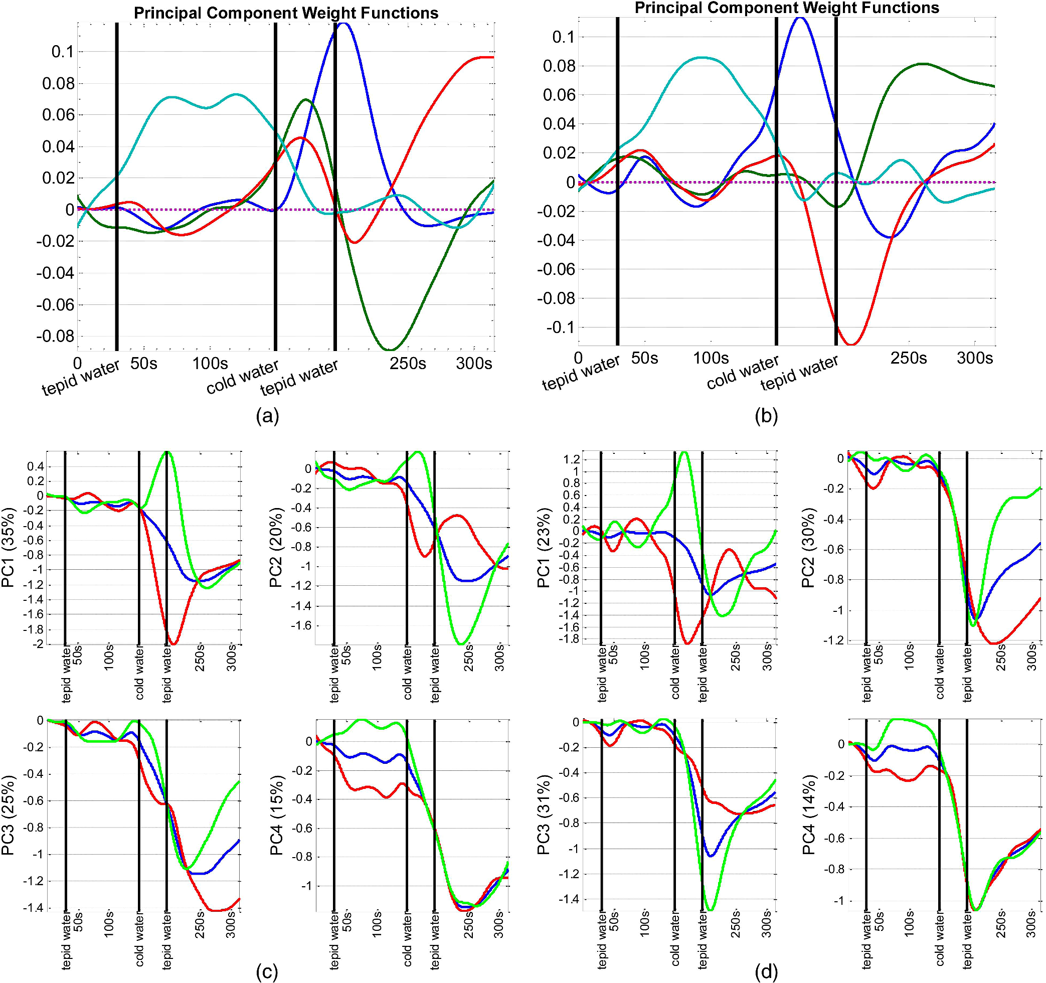

Each rotated PC weight function [Figs. 5(a), 5(b), 6(a), and 6(b)] shows variation during a brief time window compared with unrotated PC weight functions [Figs. 3(a), 3(b), 4(a), and 4(b)] that described variation over a long time span. This effect of rotation is more evident in the mean function perturbations [Figs. 5(c), 5(d), 6(c), and 6(d)].

For ${\mathrm{HbO}}_2$ data (Fig. 5), the two most important PCs that account for the largest percentage of total variability identify the evoked response during the stimulus condition and the recovery during poststimulus condition. The PC weight function associated to the stimulus condition identifies slope and amplitude variation of the evoked response and a temporal shift in the peak of response across the 20 subjects. The PC weight function associated to the poststimulus condition corresponds to amplitude and timing variation of the hemodynamic recovery curve. The two least important PCs are associated to variations in the prestimulus and end of the poststimulus conditions.

For Hb data (Fig. 6), the largest variability is observed during the poststimulus condition by PC2 and PC3 for both channels; one associated to variation in the hemodynamic settlement at the end of the poststimulus and the other one associated to variation of peak of the evoked response occurred with a delay after removal of the stimulus. The two least important PCs identified variation during the stimulus and prestimulus conditions.

3.3.

Results of fCCA

fCCA was applied to Hb and ${\mathrm{HbO}}_2$ curves to explore their interaction and shared variation. We used the cross-validation criterion proposed by Leurgans et al. to find the optimum value of the smoothing parameter ($\lambda$) for the canonical weight functions.⁴³ Based on the cross-validation results and visual inspection of plotted canonical weight functions, a $\lambda$ of ${10}^7$ for far channels and a $\lambda$ of ${10}^8$ for near channels were selected.

We present and discuss the first canonical weight functions, a.k.a. the leading weight functions, for two far channels and two near channels on the right and left sides of forehead (Fig. 7). Results for the other far channels were similar to the presented far channels.

Fig. 7

Canonical correlation analysis of Hb (blue dashed) and ${\mathrm{HbO}}_2$ (red solid) data for two “far” channels (a: right, b: left) and two “near” channels (c: right, d: left).

Figure 7 shows that the variation from the norm for Hb and ${\mathrm{HbO}}_2$ is positively correlated throughout the experiment for all channels. For the right far channel, however, the dominant mode of covariation exists in the peak and timing of Hb and ${\mathrm{HbO}}_2$ changes, with ${\mathrm{HbO}}_2$ variation being smaller and much faster than Hb response.

4.

Discussion

fDA characterizes the main features shared by a set of observations from a number of individuals. In this research, we proposed the fDA as a novel tool for the analysis of fNIRS data and showed that the fPCA is capable of decomposing the Hb and ${\mathrm{HbO}}_2$ time series during a CPT task into the experimental conditions.

Multivariate PCA has been previously used to identify the systemic interference and remove it from fNIRS measurements. Zhang et al.⁴⁴ used spatial eigenvector-based analysis of baseline activity in diffuse optical imaging. They used dozens of optodes over a large area of the cortex and showed that baseline information can be used to estimate global physiological interference during a finger tapping task and a tactile stimulus. Virtanen et al. compared PCA and independent component analysis (ICA) performance in removing superficial physiological interference during hypocapnia and hypercapnia maneuvers.⁴⁵ Instead of using a fine grid of source–detector pairs, they used two channels with short (1 cm) and far (3 cm) source-detector distances and showed that both PCA and ICA are capable of effectively removing the physiological activity from the fNIRS measurements.

fNIRS data are naturally continuous time series that are observed in discrete time. The frequency response of the hemodynamics is relatively low compared to typical fNIRS devices sampling rate and the recorded sample points are likely to be correlated. Therefore, a more accurate and effective way to look at fNIRS data is to incorporate the information that is inherent in the time order and smoothness of fNIRS data.

In traditional or standard PCA, the data are treated as vectors of discrete samples and permutation of components will not affect the analysis and thus, the time order of the physiological phenomena is irrelevant. Moreover, it is well-known that large number of measurements on each of a comparatively small number of subjects or experimental units, the so-called “large $p$, small $n$ problem,” might lead to ill-posed problems³² and also, the estimation of maximum eigenvalue might be asymptotically biased.⁴⁶ The fDA approach exploits smoothed curves and estimates a smoothed fixed covariance function to avoid the “curse of dimensionality.” The fixed covariance function solves the problem of large covariance matrices whose dimensions exceedingly increase with the sample size. Hence, fDA alternative solution for handling high-dimensional data is becoming very popular. Also, because the fDA methodology considers the entire curve as a single entity, there remains no issue regarding high correlation between repeated measurements.

fPCA is an exploratory tool to capture the principal directions of variation in the population and dimension reduction. Our study provides a good understanding of the variation in the population structure of Hb and ${\mathrm{HbO}}_2$ at different conditions of a CPT. Our observations are summarized as follows:

In a secondary exploration, we investigated the association between Hb and ${\mathrm{HbO}}_2$ variability using fCCA. We were interested in the dominant modes of correlation between Hb and ${\mathrm{HbO}}_2$. Results demonstrated an overall positive correlation between Hb and ${\mathrm{HbO}}_2$ variation through the CPT experiment. However, for a right far channel, there was an evident time shift in the Hb response relative to ${\mathrm{HbO}}_2$. In general, fCCA gives a broad view of the interaction between two variables. The identified patterns of covariation give important directions for further investigation of interaction between Hb and ${\mathrm{HbO}}_2$ in a particular experimental setting.

Feature selection for the preliminary study of CPT data published elsewhere was done empirically.³⁶ By visual inspection of the Hb and ${\mathrm{HbO}}_2$ data, we observed that the amplitude and slope of the evoked hemodynamic response were quite variable between subjects, and we chose two features based on these characteristics for statistical analyses.³⁶ However, empirical search did not give any information regarding the power of these features for explaining variability without running comprehensive statistical analyses. However, fPCA aids a straight feature selection by characterizing the geometry of curves as a set of principal directions of variation. Exploratory functional analysis of CPT data gave us new insight into our dataset by: (1) explicit estimation of PCs explaining the highest variability in the dataset, (2) calculation of the percentage of total variability explained by each component, and (3) study the covariation of Hb and ${\mathrm{HbO}}_2$ throughout a CPT experiment. We showed that fPCA could successfully discriminate different phases of the hemodynamic response during a CPT experiment and interestingly, it identified two components for the poststimulus condition: an early component associated to variation in the hemodynamic recovery and a late component associated to the hemodynamic settlement. More importantly, it described inter-subject variations in the dynamic of the response, such as slope of the evoked response and slope of the recovery curve. In addition to this qualitative information, fPCA provided quantitative measures of the importance and weight of each of these features based on the percentage of total variability explained by that feature; for instance, experimental manipulations that created the largest variation among the dataset were identified to be the stimulus and early poststimulus conditions. Extracting such detailed information from the raw data (Figs. 1 and 2) was impractical, if not impossible. For future studies, we will exploit these findings for further statistical analysis of CPT data as well as designing new protocols according to the extracted features (e.g., how much time would be necessary for the hemodynamic recovery/settlement after a cold stimulus).

In the context of brain imaging studies, as Tian³³ pointed out in her review article, fPCA can play a critical role in research involving a stimulus-response paradigm when the onset, duration, amplitude, and/or speed of the evoked brain activity is unknown or uncertain, such as in a decision-making process or an emotional reaction. As an exploratory technique, fPCA does not make any a priori assumption on the form and timing of the waves of neural activity and this key property makes fPCA application particularly relevant in neuroscience studies employing fNIRS as well as other neuroimaging tools such as electro-encephalography, fMRI, and magneto-encephalography.³³

After exploratory steps, one can extract more pertinent information. For instance, fPCA is a good tool for computing proximities between curves in a reduced dimensional space. Using such a distance measure, one can investigate whether the curves are similar or can be split into several classes.

Due to inherent interaction between the autonomic nervous system and central pain processing system, researchers try to assess the individuals’ perception of pain through physiological signs. Hemodynamic changes at the skin and major arteries have been investigated to study the sympathetic response to a noxious stimulus.^47–49 In this exploratory study, we attempted to learn what feature of response to a cold noxious stimulus is most variable among control subjects. We showed that the PCs explaining the variability in the CPT data and their weight varied between Hb and ${\mathrm{HbO}}_2$ parameters and channels. This information may be helpful to decide which parameter and/or channels are most associated with the hypothesized effect, for example, in brain mapping studies. With the CPT experiment, we previously showed that the amplitude and timing of the evoked response of ${\mathrm{HbO}}_2$ was correlated with subjects’ report of the pain intensity.³⁶ Through the results of this research, we also learned about importance of the dynamics of the evoked response to a CPT as revealed by fPCA. In another study, we used this information and considered the derivatives of ${\mathrm{HbO}}_2$ curves during a pain tolerance test using CPT. Results confirmed that the amplitude and timing of the peak of the first and second derivative of the ${\mathrm{HbO}}_2$ response right after hand immersion in cold water is a very robust feature. In future, we will use this knowledge to better understand the physiology of pain through explaining some of the observed variations by known factors such as age, gender, or information about whether the subjects are high/low tolerance to that specific stimulus.

The observed modes of variation and covariation patterns can help improve design of fNIRS studies for pain research in particular and for other experiments in general. This study was preliminary but opens an interesting avenue for future research. Without a good understanding of population structure, it would not be feasible to formulate and study physiological phenomena and identifying variability is the first step in this direction.