|
|
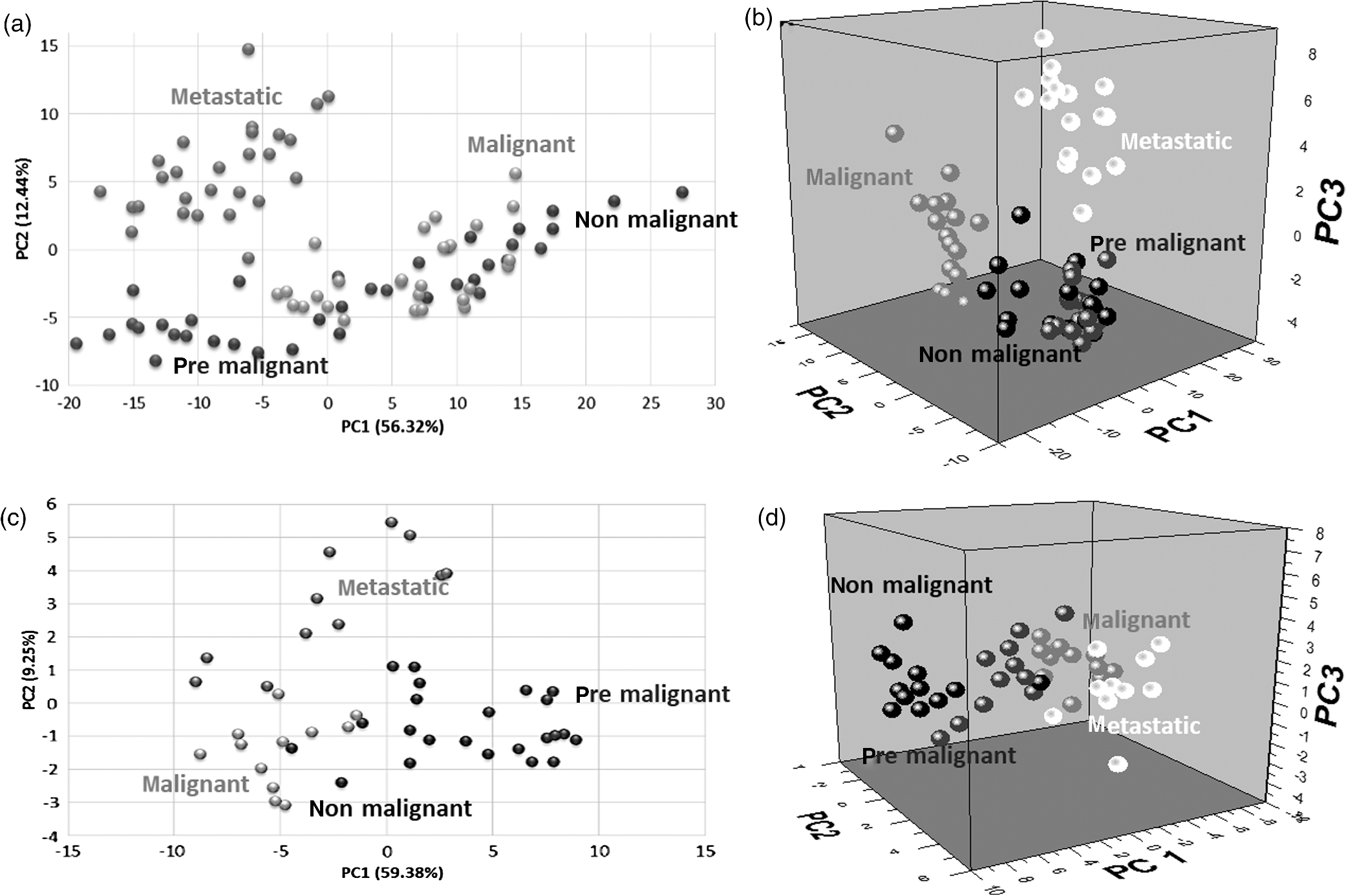
1.IntroductionRaman spectroscopy is an analytical technique based on inelastic scattering of light, capable of providing chemical specificity with a suitable enhancement down to a single molecule resolution.1–5 The presence of specific chemical bond diversity on cell surfaces relates to the diversity of cell surface composition consisting of carbohydrates, proteins, and lipids among others.3,5,6 With the surface-enhanced Raman spectroscopy, subcellular fingerprinting (e.g., nucleic acids and amino acids) has been possible, enabling Raman spectroscopy as a viable method for the classification of complex in vivo biomolecular analysis and monitoring.4 Raman spectroscopy has been shown to be accurate in differentiating nonmalignant and malignant entities, such as in skin lesions,5,7 epithelial breast cancer cells,6 gastrointestinal, colorectal, and lung cancer cells.8–11 The focus of our study is on breast cancer using a three-dimensional (3-D) cell culture model system that mimics an in vivo condition. Breast cancer is a lethal heterogeneous disease12 with diversity within and between tumors and also among patients.13 The complexity of this disease poses a challenge in cancer diagnosis, prognosis, and in the assessment of populations that have developed a therapeutic resistance. Therefore, there is a need for robust diagnostic and classification tools that are reproducible and have clinical potential.12 Although Raman spectroscopy has been used for ex vivo and in vivo classification of breast cancer,4,14–19 most of the past work predominantly focused only on the differentiation of nontumorigenic and tumorigenic cells, while few address stage-based classification (from nonmalignant, premalignant, malignant, to metastatic). Furthermore, most of the past work using Raman spectroscopy for breast cancer classification used two-dimensional (2-D) cell culture models, where the extracellular matrix, a critical factor in cell phenotype regulation, is unaccounted for.20 Under 2-D conditions, cells tend to lose part of their context due to the absence of an extracellular environment and other characteristics necessary for cell-to-cell communication, growth, and differentiation. The work presented here is the first to evaluate Raman spectroscopy as a potential tool for cancer staging using 3-D breast cancer model with elastic net regularized regression analysis to reveal the relationship between characteristic Raman fingerprint and the stage of cancer. We tested our hypothesis that Raman spectroscopy is a viable tool for breast cancer classification using 2-D and 3-D cell culture models in conjunction with the application of principal component analysis (PCA), partial least squares discriminant analysis (PLS-DA), and elastic net analysis. Our work addresses the: (1) potential of Raman spectroscopy to differentiate cancer cells at different stages of tumorigenesis; (2) classification efficacy to differentiate cells at different stages of the disease; and (3) determination of key chemical components that account for the differences observed in the cells at different stages of malignant transformation. Spectral analysis from elastic net is supported by statistical methods, PCA, and PLS-DA. 2.Materials and Methods2.1.Cancer Cell LinesThe MCF10 model is a panel of isogenic human breast epithelial cell lines, namely MCF10A (nonmalignant), MCF10AneoT (premalignant), MCF10CA1h (malignant, but not metastatic), and MCF10CA1a (metastatic), each at a distinct stage of cancer progression.21 Spontaneously immortalized, nonmalignant breast epithelial MCF10A cells were developed from a human benign fibrocystic breast disease specimen. Introduction of the H-Ras oncogene in MCF10A cells gave rise to the premalignant MCF10AneoT cells which were serially passaged in immunocompromised mice resulting in the accumulation of tumor-promoting mutations. This led to the development of human tumor xenografts with varying degree of malignancy, ultimately giving rise to various MCF10CA1 clones. MCF10CA1h cell line consists of well-differentiated tumor cells that are malignant, but not metastatic, whereas MCF10CA1a line consists of poorly differentiated cells that are metastatic in immunocompromised mice.21–26 These cell lines have been extensively characterized by cytogenetic and microarray analysis and have been used to study key signaling pathways and molecular and genetic events in tumorigenesis.27–29 Since the cell lines in the MCF10 series are isogenic and represent the major stages of breast cancer progression, they were an ideal choice for this study. All the cell lines were obtained from Barbara Ann Karmanos Cancer Institute (Detroit, Michigan). 2.2.Cell Lines Growth ConditionsMCF10A and MCF10AneoT cells were cultured and maintained in Dulbecco’s modified Eagle’s medium nutrient mixture F-12 HAM [with 15 mM 2-[4-(2-hydroxyethyl)piperazin-1-yl]ethanesulfonic acid (HEPES), , pyridoxine, and l-glutamine; Sigma] supplemented with 5% horse serum (Sigma), choleratoxin (Sigma), EGF (SAFC Biosciences, St. Louis, Missouri), insulin (Sigma, St. Louis, Missouri), and hydrocortisone (Sigma). MCF10CA1h and MCF10CA1a cells were grown in Dulbecco’s modified Eagle’s medium nutrient mixture F-12 HAM (with 15 mM HEPES, , pyridoxine, and l-glutamine; Sigma) supplemented with 5% horse serum. All the cells were cultured in 5% incubator at 37°C. 2.3.Sample PreparationFor 2-D culture, the cells were cultured in a flask (Nunc, Rochester, New York) to reach 80% confluency. The cells were trypsinized and 0.5 mL of the cell suspension was added to 35-mm tissue culture dishes (Falcon, Franklin lakes, New Jersey) with gold slides placed inside the dish. Subsequently, 2.5 mL of culture medium was added and the cells were cultured to reach 80% confluency. By using this method, the cells were grown both on the surface of the gold slide and in the tissue culture dish. The slides were subsequently taken out and placed into a new tissue culture dish. The cells on the gold slide were rinsed twice with Gibco phosphate-buffered saline (PBS) at 37°C (pH 7.4, Life Technologies, Carlsbad, California) to remove the remaining culture medium and placed in 1.3 mL PBS to prevent the cells from drying out during measurement. The main steps involved in sample preparation are schematically illustrated in Fig. 1. Fig. 1Schematic of a two-dimensional (2-D) and three-dimensional (3-D) cell culture systems: (a) 2-D; (b and c) 3-D culture models (top) and 3-D cell sample preparation (bottom). 3-D cell lines were first cultured in a 24-well plate in an embedded model, washed, and a piece of gel was then taken, placed onto the gold slide for Raman measurement that followed. 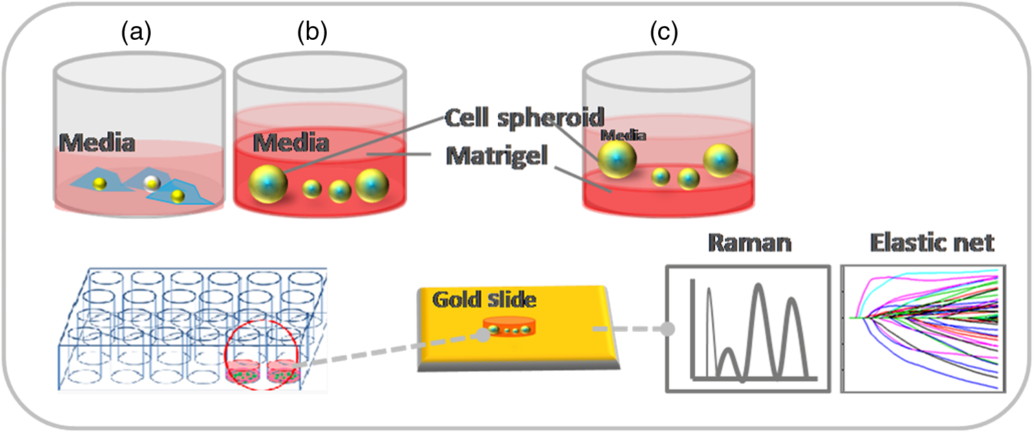 In Fig. 1, the 2-D cell culture and the two common types of 3-D cell culture models are shown: Fig. 1(b) shows, an “embedded model” in which a mixture of cell suspension with liquefied Matrigel is prepared as a first step followed by the addition of culture media after the solidification of the Matrigel. The second method for 3-D cell culture preparation is the “on-top model,” Fig. 1(c), where solidified Matrigel is used as a substratum before adding the mixture of culture media and cell suspension. Here, the cells adhere to the surface of the Matrigel and initiate the formation of clusters on the surface. In this work, in order to keep the cell clusters alive during measurement, the embedded model was adopted as the surrounding Matrigel protects the specimen from drying out due to the evaporation of the liquid medium during measurement. For 3-D cell culture, were resuspended in 10 μL of growth medium and added to 150 μL Matrigel basement membrane matrix (BD Biosciences, San Jose, California) on ice. The mixture of cells and Matrigel was evenly layered in a 24-well tissue culture treated plate (BD Falcon, Franklin lakes, California) and incubated in a 5% incubator at 37°C for 30 min. After 30 min, 1.5 mL of prewarmed growth medium was gently layered from the side of the well onto the matrix/cell mixture. The cells were maintained in the 3-D culture at 37°C with 5% for 5 days with the medium replaced every 2–3 days. The cells were allowed to form 3-D spheroids and then imaged using the Ziess AxioObserver microscope with Axiovision software. The cells were analyzed after 5 days in the 3-D culture. The culture medium was removed and the cells were washed twice with PBS to remove the remaining culture medium; PBS in the well was subsequently removed and a section of the Matrigel with 3-D cell spheroids was removed with a spatula. The Matrigel was placed on the gold slide for the spectral analysis, and the remaining Matrigel was kept in the incubator for further measurements. 2.4.Data Collection by Raman SpectrometerThe Senterra Confocal Raman Spectrometer (Bruker Optics Inc., Billerica, Massachusetts), fitted with a objective was used. The 50 μm pinhole was activated to remove stray light from the out-of-focus plane. Cells grown in 2-D and 3-D cultures are shown in Figs. 2(a) and 2(b), respectively. A 633 nm He-Ne laser with 20 mW power was used for excitation and an integration time of 45 s was used for Raman spectra acquisition. During measurement, the cells attached to the gold slide displayed a spindle form, thus no tissue damage was observed under the laser conditions used. This can be explained by the fact that cells gradually display a round shape instead of the spindle shape when dying. The schematic of the optical layout is illustrated in Fig. 2(c).30–34 Fig. 2Schematic of sampling for 2-D and 3-D culture systems: (a) five spots were chosen for data collection in each 2-D cell, (b) 15 spots distributed throughout the spheroid were chosen in the 3-D spheroid, and (c) schematic of the optical layout of the Senterra Confocal Raman spectrometer: the laser is directed through a neutral density filter to excite the sample through the objective and the scattered photons are collected by the same objective. A pinhole is used to detect photons from the plane of focus. 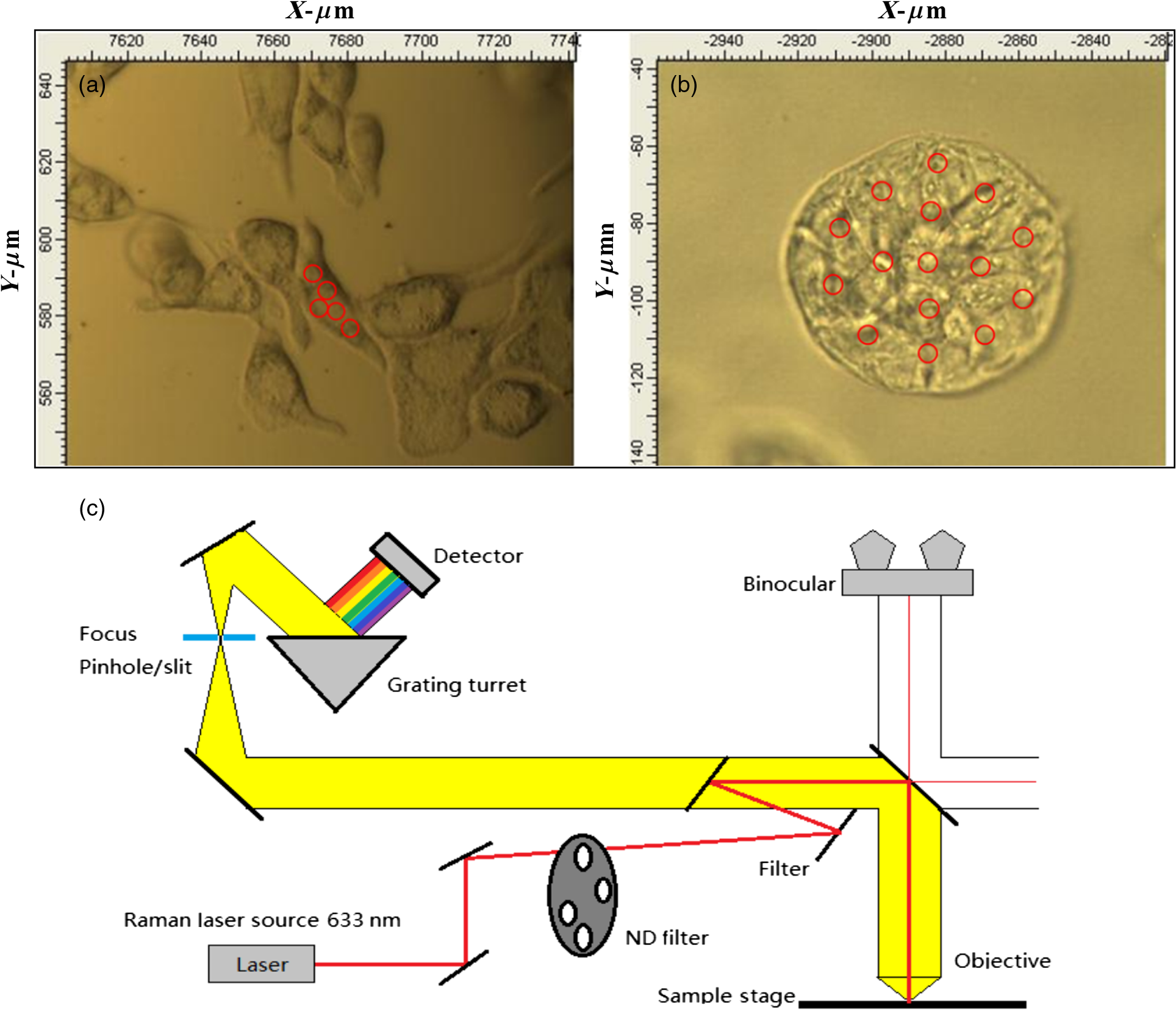 For both 2-D and 3-D cell samples, three independent biological replicates were performed. In the 2-D cell cultures, 10 cells were measured in each cell, five measurements were made by choosing different spots (one is at the center) to ensure that all components of the cell were probed. For the 3-D cell sample, since the cells formed clusters, called spheroids, the samples were studied as spheroids rather than as single cells. In each biological replicate, four spheroids were chosen for analysis and 15 different spots were chosen across the spheroid (one center point and four spots surrounding this spot and 10 spots at the exterior) for measurement in each sample. The data collection and analysis for both 2-D and 3-D cultures are noted below. 2.5.Data PretreatmentData analysis was done using R software. The raw spectra were first processed to accommodate the range of the Raman shift which contains most of the biological fingerprints.17–19 The spectra were baseline corrected by fitting polynomials using the R software to remove the effects of fluorescence and allow for the acquisition of spectra with band edges up to the theoretical baseline to visualize minor peaks. The spectra obtained were normalized to ensure that the area under the curve was unity, for further evaluation. 2.6.Statistical AnalysisThe statistical analysis of this study was conducted in three steps. First, PCA was applied to assess data variability and to detect outliers. These outliers were removed from the data set and consequently not included in the subsequent statistical techniques. In sequence, PLS-DA, a well-established classification technique was applied to the data to actually classify the samples based on their cell lines. Beyond the development of classification models, in a third step, an interpretation of the main differences between cells in different stages of cancer was attempted by elastic net,35 providing an interesting visualization of specific compounds associated with this progression. Elastic net is a version of penalized least squares that combines both Ridge and Lasso regressions. In this technique, the wavenumbers that reveal an explicit relationship with the different stages of tumor progression are selected with their respective coefficient estimates that represent the extent of contribution of each of these wavenumbers to the correct classification of each cell line. 2.6.1.Exploratory analysis and outlier removalPCA is an exploratory multivariate analysis technique that projects the data matrix to a lower-dimensional space spanned by the loading vectors. The loading vectors corresponding to the largest eigenvalues are retained to optimally capture the variance of the data and to minimize the effect of random noise.36 The goodness-of-fit between the data and the model can be calculated using the residual matrix and statistics that measure the distance of a sample from the new space of the PCA model.36 Hotelling’s statistics indicates how far the estimated sample by the PCA model is from the multivariate mean of the data, thus these statistics provide an indication of variability within the normal subspace.37 The combination of and tests is used to detect the remaining abnormal observations. Given the level of significance for the and statistics, measurements with or values over the threshold are classified as outliers.37 After the elimination of the outlier spectra from the model, the procedure was continually repeated until no outliers could be identified. The software MATLAB (The MathWorks, Co., Natick, Massachusetts) and the computational package PLS_Toolbox (Eigenvector Research, Inc., Wenatchee, Washington) were employed. All data were mean centered prior to PCA. 2.6.2.Classification of cells in different stages of cancerPLS-DA is a parametric and linear model and one of the most applied techniques for the classification of spectral data. The basics of PLS-DA consist of the application of a partial least squares regression model with variables which are indicators of groups. The second step of PLS-DA is to classify observations from the results of PLS regression on the indicator variables.38 MATLAB (The MathWorks, Co., Natick, Massachusetts) and the computational package PLS_Toolbox (Eigenvector Research, Inc.) were employed for PLS-DA analysis. In both 2-D and 3-D models, spectral data were divided into calibration (75%) and validation (25%) data sets. Cross-validation (comprising of leave-one-out analysis) was applied to estimate the performance of the models and to choose the optimal number of latent variables. The predictability of the resulting models was evaluated based on the classification error for the validation set. Sensitivity is defined as the proportion of true positives that were classified as positive, and specificity represents the proportion of true negatives that were classified as negative. The later parameters were calculated as follows: 2.6.3.Variable selectionElastic net35 was applied using the glmnet package of the R software that fits generalized linear models via penalized maximum likelihood. Samples were randomly separated into training (75%) and validation (25%) data sets. The regularization parameter lambda causes coefficient shrinkage, minimizing the residual sum of squares. In order to obtain the lambda value that gives a minimum cross-validated error, leave-one-out cross-validation was performed. In sequence, multinomial logistic models were fitted with the training data set at values ranging from 0 to 1, in steps of 0.25. The parameter controls the mixing between Ridge and Lasso regressions. Ridge regression () imposes an -penalty to the model resulting in a coefficient shrinkage, while Lasso regression () imposes an -penalty which expects many predictors to be close to zero and a small subset to be nonzero, providing automatic variable selection.39 Elastic net () provides both coefficient shrinkage and variable selection. The developed models were used to predict the degree of classification as well as validation using the validation data set. The -value that provided the higher predictability based on the lowest classification errors was considered as the best-fit model. The discriminant wavenumbers from the best-fit model and their respective coefficient estimates were then extracted. 3.Results3.1.Raman SpectraFigure 3 shows the average Raman spectra from a total of 150 spectra for the 2-D [Fig. 3(a)] and 180 spectra for the 3-D [Fig. 3(b)] cell culture model in the range . Each spectrum was previously baseline corrected and normalized as described in Sec. 2. Standard deviation information is also provided. Fig. 3Mean Raman spectra of (a) 2-D and (b) 3-D cell cultures of benign, MCF10A (black), premalignant, MCF10AneoT (dark gray), malignant, MCF10CA1h (medium gray), and metastatic MCF10CA1h (light gray). Standard deviation is provided. 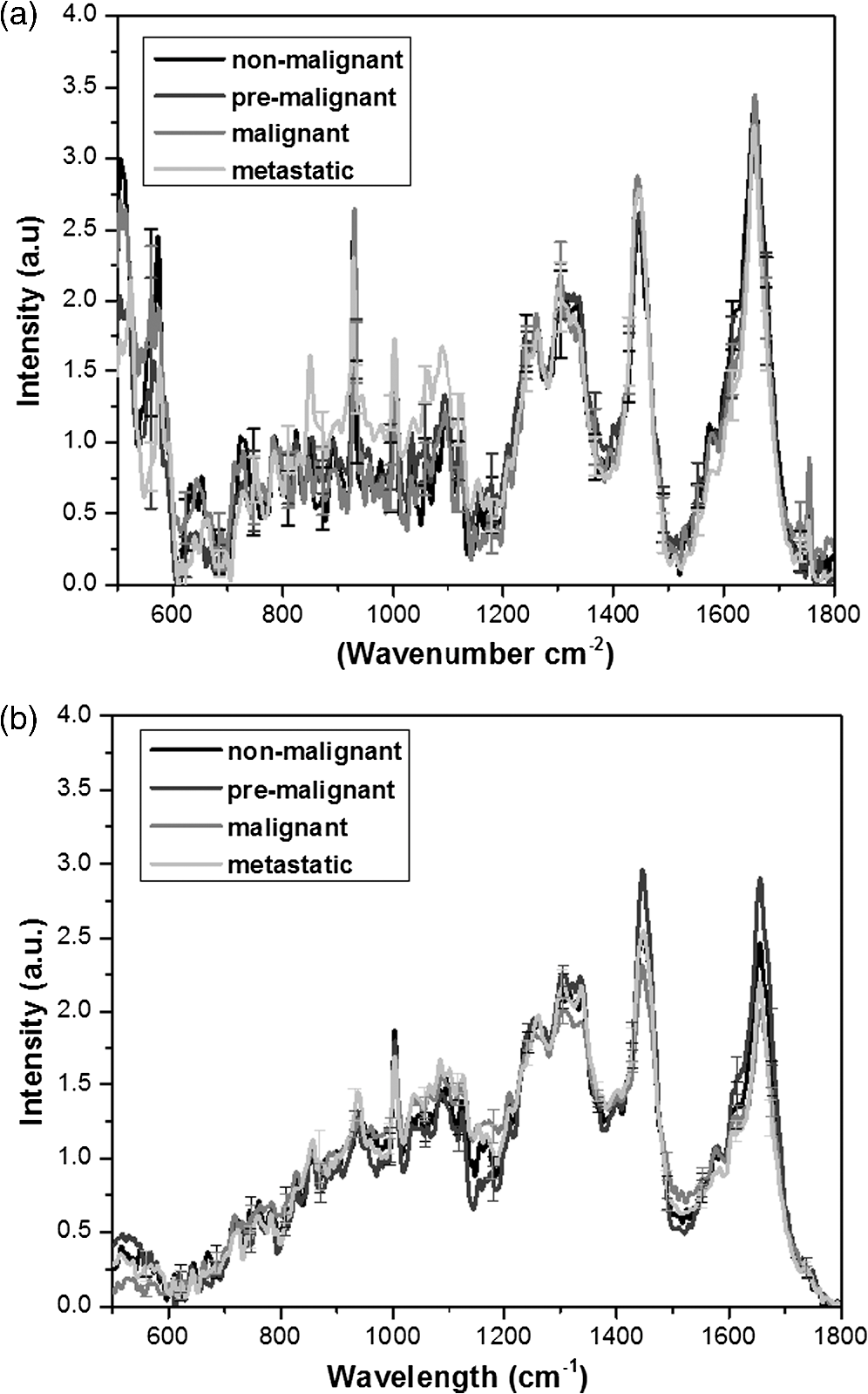 Despite the similarities between the 2-D and the 3-D spectra, especially in the region 800–1150, 1200–1350, and , differences could be noted in the spectral window , and peaks in the 2-D cell culture samples merged into a broad shoulder in the 3-D cell systems. Spectra from the metastatic (MCF10CA1a) cell lines had a higher intensity than other cell lines in the region . This trend was observed in both the 2-D and 3-D cell culture samples, although it is more evident in the 2-D cells. In the 3-D system, it is evident that premalignant samples show higher intensity than other cell lines in the 1451 and peaks, and nonmalignant samples show a higher intensity than malignant and metastatic at the peak. An opposite trend was observed in nonmalignant and premalignant at the shoulder, where the 2-D samples exhibited intensity in the following order; , while in the 3-D system the premalignant samples show higher intensity than nonmalignant. However, based only on the visual observation of the spectra, it is not possible to arrive at major conclusions, especially when considering the standard deviation between each cell line. In the 2-D model the minimum–maximum values of the standard deviation in the nonmalignant, premalignant, malignant, and metastatic cell lines were 0.06–1.22, 0.05–1.04, 0.07–0.57, and 0.05–0.57, respectively; in the 3-D models, these values were 0.03–0.21, 0.02–0.24, 0.02–0.18, and 0.02–0.31, respectively. A discussion on the main differences between the spectra of each cell line will be conducted in the next sections supported by statistical analysis. 3.2.Exploratory Analysis and Outlier Removal by PCAUsing PCA, the original high-dimensional spectral data set containing chemical and biological characteristics of the cancer cell lines was projected to a low-dimensional space where the first principal components (PCs) explained most of the variance between the samples. Samples with or statistical values over the threshold were classified as outliers and removed from the data set. The procedure was repeated until no outliers were identified. For the 2-D cell culture models, 19 observations from the original data set containing 110 observations were identified as outliers. On the other hand, two from the original 48 observations from the data set of the 3-D cell culture models were identified as outliers and removed from the data set. The resulting scatter plots obtained by PCA analysis are shown in Fig. 4. For the 2-D cell culture, the first two PCs clearly separated metastatic cells from the other cell lines [Fig. 4(a)]. The inclusion of the third PC provides a 3-D scatter plot that also discriminates malignant, but nonmetastatic from the rest of the group, as shown in Fig. 4(b). Thus, based on the variance of the spectral data from the 2-D cell culture, the two stages of cancer could be separated into two clusters while nonmalignant and premalignant were clustered together. In the case of the 3-D cell culture, the first two PCs displayed four clusters of the cell lines, although some overlap was observed [Figs. 4(c) and 4(d)]. 3.3.Classification Based on PLS-DAResults from our exploratory analysis indicate that Raman spectra can provide sufficient information to develop classification models for different stages of cancer cells. Thus, PLS-DA was further applied to the spectral data with the purpose of obtaining classification models for assigning samples to categories. Based on leave-one-out cross-validation, five and six latent variables were chosen and employed in the development of the 2-D and 3-D cell culture models. Table 1 summarizes the classification results obtained. Accurate classification was obtained for both the 2-D and 3D cell culture models with the accuracy up to 100% for malignant and premalignant in both models. The sensitivity in the validation set for nonmalignant cells is lower in 2D models compare to the sensitivity of nonmalignant cells in 3D models. The overall classification error for the 3-D model is considered to be lower than the 2-D model, especially for the classification of nonmalignant cells. Table 1Summary of PLS-DA prediction results of the model developed for classification of cancer cell lines.
Due to the fact that relatively small number of samples was used in the development of the 3-D model, a lower number of latent variables would be preferred in order to guarantee the stability and robustness of the model. However, the number of latent variables employed reflects the complexity of the samples being analyzed, and a reduction in this number leads to an accuracy decay. Nevertheless, Table 2 shows the classification results for the 2-D and 3-D models constructed with one to three latent variables, respectively. Satisfactory results were obtained with only three latent variables for both the 2-D and 3-D models. Table 2PLS-DA prediction results of the models developed for the classification of 2-D and 3-D cancer cell lines (number of latent variables are included).
3.4.Variable Selection by Elastic NetElastic net was applied in this study for visualization of the discriminating wavenumbers and to know what extent these wavenumbers contributed to the correct classification of each cell line. Multinomial logistic models were developed by varying the parameter . Perfect statistical classification was achieved for an value of 0.5 in both the 2-D and 3-D systems. The coefficient estimates from the developed models were then extracted.33 As demonstrated in Fig. 5, each stage of breast cancer was identified by specific coefficient estimates in both the 2-D and 3-D models; overall, 3-D cells exhibited fewer coefficients for each stage. Premalignant cells were identified by the prominent positive peak at and a negative peak at in both 2-D and 3-D, but only in the 3-D model a prominent positive peak appeared at . High negative coefficients for nonmalignant cells were observed at in the 3-D model. Premalignant, malignant, and metastatic stages were identified by different coefficient estimates in the 2-D and 3-D cell cultures, although the premalignant state yielded a negative peak at . A prominent negative peak for the premalignant cell line was observed at in the 2-D model. Malignant cells were identified by a strong positive peak at in the 2-D model and strong negative peaks at 555 and in the 3-D and 2-D models, respectively. Higher peaks associated with the metastatic cell line were mostly observed in the 3-D model, with a strong positive peak at and negative peaks in the following regions: 732, 1006, 1236–1240, and . Fig. 5Elastic net coefficient estimates for for (a) 2-D and (b) 3-D cell culture models. A peak indicates that the correct classification of spectra is associated with the corresponding spectral region. A positive peak indicates higher intensity than other cell lines; a negative peak indicates lower intensity.  We examined each of the nonzero coefficient estimates and, based on the existing work, tentative assignment of these coefficients to chemical compounds were made that relate to specific regions in the Raman spectrum (Table 3). Table 3Coefficient estimates obtained from elastic net and its tentative peak assignment from the literature (Refs. 32–40).
4.Discussion4.1.Raman Spectroscopy for Breast Cancer ClassificationBased on our results (Fig. 4 and Table 1), the methods and analysis procedures used for classifying 3-D models using PCA and PLS-DA has a similar trend as the 2-D classification, providing evidence that the methods developed are robust.38 Based on PLS-DA, excellent results were achieved in the classification of metastatic and malignant cells (specificity 100%, sensitivity 100%); however, lower sensitivity was observed when classifying nonmalignant cells in the 2-D model compared to that of the 3-D system. Low sensitivity (60%) and high specificity (100%) for nonmalignant cells indicate the possibility of nonmalignant cells to be classified as premalignant cells in the 2-D model; however, malignant and metastatic stages would not be classified as nonmalignant. Higher sensitivity was achieved for nonmalignant cells in the 3-D model, which suggests that the change in the extracellular matrix environment and interaction plays a key role in the development of premalignancy in breast cancer.40 Malignant stages are accurately classified in both the 2-D and 3-D models; suggesting that the malignant characteristic is preserved in both the 2-D and 3-D cell culture models. 4.2.Variable Selection by Elastic NetAlthough PLS-DA alone can provide satisfactory classification, this technique cannot reveal sparse variables that contribute to the classification of each cell line, since each of the latent variables used in the development of the PLS-DA models is a linear combination of several original variables, representing a problem in terms of variable selection. Elastic net was used in this study to solve the aforementioned problem, making the data more succinct and simpler, and providing a good interpretation of the model.41 More importantly, elastic net reveals the relationship between breast cancer stages and discriminating wavenumbers that give the most contribution to the correct classification of each cell line. This knowledge will be useful in understanding the underlying biomolecular processes in the breast cancer tumorigenesis. Based on our results, extracellular matrix plays an important role in the genesis of malignancy. Prominent coefficients indicate that nonmalignant cells exhibit a high content of polysaccharide and the lowest aromatic amino acid content (Table 3),42,43–51 which is in agreement with the previous report which implicates lipid genesis in neoplastic transformation52,50 and characteristic aromatic amino acid content during malignancy development.53,51 High lipid and nucleic acid content are characteristics of metastatic cells, while high aromatic content and lower polysaccharide composition are characteristic of malignant cells.42–53 These results suggest that lipid, polysaccharide, and aromatic amino acid constituents can serve as potential biomarkers in monitoring tumor progression. 5.ConclusionOur study presents the first application of Raman spectroscopy to classify 3-D breast cancer cell culture models and to discriminate between the nonmalignant, premalignant, malignant, and metastatic stages of breast cancer. The 3-D model is unique because it accounts for the extracellular matrix and is a better representative of an in vivo environment than the 2-D cell cultures. Hence, our work presents an important step in translation. Analysis of Raman spectra using elastic net indicates that the tools developed can accurately discriminate the premalignant from nonmalignant with the specificity and sensitivity nearing 100%. We also show that Raman spectroscopy can differentiate the two forms of malignant cancer; metastatic, and nonmetastatic. Evaluation of the spectra indicates that the polysaccharide, lipid, nucleic acid, aromatic amino acid, and extracellular matrix components are involved in the staging of breast cancer. Our methods suggest that the incorporation of Raman spectroscopy and statistical techniques, such as PLS-DA and elastic net, makes the classification of cells within the tissues possible with a high degree of accuracy. AcknowledgmentsPartial funding from the Purdue University Center for Cancer Research innovation grant and the Clinical Translational Sciences Institute (CTSI) of Indiana is acknowledged. Financial support from the Brazilian Government Agency CNPq for AC is appreciated. The authors thank Sarah Voisin and Kate Stephen, former students in Irudayaraj group for assistance in the R software. ReferencesK. LarssonR. P. Rand,
“Detection of changes in the environment of hydrocarbon chains by Raman spectroscopy and its application to lipid–protein systems,”
Biochim. Biophys. Acta, 326
(2), 245
–255
(1973). http://dx.doi.org/10.1016/0005-2760(73)90250-6 BBACAQ 0006-3002 Google Scholar
W. E. MoernerL. Kador,
“Optical detection and spectroscopy of single molecules in a solid,”
Phys. Rev. Lett., 62
(21), 2535
–2538
(1989). http://dx.doi.org/10.1103/PhysRevLett.62.2535 PRLTAO 0031-9007 Google Scholar
E. C. Le RuP. G. Etchgoin,
“Single-molecule surface-enhanced raman spectroscopy,”
Ann. Rev. Phys. Chem., 63 65
–87
(2012). http://dx.doi.org/10.1146/annurev-physchem-032511-143757 ARPLAP 0066-426X Google Scholar
K. Kneippet al.,
“Single molecule detection using surface-enhanced Raman scattering (SERS),”
Phys. Rev. Lett., 78
(9), 1667
–1670
(1997). http://dx.doi.org/10.1103/PhysRevLett.78.1667 PRLTAO 0031-9007 Google Scholar
R. S. DasY. K. Agrawal,
“Raman spectroscopy: recent advancements, techniques and applications,”
Vib. Spectrosc., 57
(2), 163
–176
(2011). http://dx.doi.org/10.1016/j.vibspec.2011.08.003 VISPEK 0924-2031 Google Scholar
C. Yuet al.,
“Characterization of human breast epithelial cells by confocal Raman microspectroscopy,”
Cancer Detect. Prevent., 30
(6), 515
–522
(2006). http://dx.doi.org/10.1016/j.cdp.2006.10.007 CDPRD4 0361-090X Google Scholar
M. Gniadeckaet al.,
“Distinctive molecular abnormalities in benign and malignant skin lesions: studies by Raman spectroscopy,”
Photochem. Photobiol., 66
(4), 418
–423
(1997). http://dx.doi.org/10.1111/php.1997.66.issue-4 PHCBAP 0031-8655 Google Scholar
K. Chenet al.,
“Diagnosis of colorectal cancer using Raman spectroscopy of laser-trapped single living epithelial cells,”
Opt. Lett., 31
(13), 2015
–2017
(2006). http://dx.doi.org/10.1364/OL.31.002015 OPLEDP 0146-9592 Google Scholar
J. R. Mourantet al.,
“Biochemical differences in tumorigenic and nontumorigenic cells measured by Raman and infrared spectroscopy,”
J. Biomed. Opt., 10
(3), 031106
(2005). http://dx.doi.org/10.1117/1.1928050 JBOPFO 1083-3668 Google Scholar
X. L. Yanet al.,
“Raman spectra of single cell from gastrointestinal cancer patient,”
World J. Gastroenterol., 11
(21), 3290
–3292
(2005). WJGAF2 1007-9327 Google Scholar
K. Chenet al.,
“Near‐infrared Raman spectroscopy for optical diagnosis of lung cancer,”
Int. J. Cancer, 107
(6), 1047
–1105
(2003). http://dx.doi.org/10.1002/(ISSN)1097-0215 IJCNAW 1097-0215 Google Scholar
L. Hutchinson,
“Breast cancer: challenges, controversies, breakthroughs,”
Nat. Rev. Clin. Oncol., 7
(12), 669
–670
(2010). http://dx.doi.org/10.1038/nrclinonc.2010.192 NRCOAA 1759-4774 Google Scholar
K. Polyak,
“Heterogeneity in breast cancer,”
J. Clin. Invest., 121
(10), 3786
–3788
(2011). http://dx.doi.org/10.1172/JCI60534 JCINAO 0021-9738 Google Scholar
A. S. Hakaet al.,
“Diagnosing breast cancer by using Raman spectroscopy,”
Proc. Natl. Acad. Sci. U. S. A., 102
(35), 12371
–12376
(2005). http://dx.doi.org/10.1073/pnas.0501390102 PNASA6 0027-8424 Google Scholar
B. Brożek Płuskaet al.,
“Breast cancer diagnostics by Raman spectroscopy,”
J. Mol. Liq., 141
(3), 145
–148
(2008). http://dx.doi.org/10.1016/j.molliq.2008.02.015 JMLIDT 0167-7322 Google Scholar
C. Matthäuset al.,
“New ways of imaging uptake and intracellular fate of liposomal drug carrier systems inside individual cells, based on Raman microscopy,”
Mol. Pharm., 5
(2), 287
–293
(2008). http://dx.doi.org/10.1021/mp7001158 MOPMA3 0026-895X Google Scholar
Z. MovasaghiS. RehmanD. I. U. Rehman,
“Raman spectroscopy of biological tissue,”
Appl. Spectrosc. Rev., 42
(5), 493
–541
(2007). http://dx.doi.org/10.1080/05704920701551530 APSRBB 0570-4928 Google Scholar
D. Zhanget al.,
“Gold nanoparticles can induce the formation of protein-based aggregates at physiological pH,”
Nano Lett., 9
(2), 666
–671
(2009). http://dx.doi.org/10.1021/nl803054h NALEFD 1530-6984 Google Scholar
N. StoneP. Matousek,
“Advanced transmission Raman spectroscopy: a promising tool for breast disease diagnosis,”
Cancer Res., 68
(11), 4424
–4430
(2008). http://dx.doi.org/10.1158/0008-5472.CAN-07-6557 CNREA8 0008-5472 Google Scholar
M. J. BissellD. C. RadiskyA. Rizki,
“The organizing principle: microenvironmental influences in the normal and malignant breast,”
Differentiation, 70
(9–10), 537
–546
(2002). http://dx.doi.org/10.1046/j.1432-0436.2002.700907.x DFFNAW 0301-4681 Google Scholar
S. J. Santneret al.,
“Malignant MCF10CA1 cell lines derived from premalignant human breast epithelial MCF10AT cells,”
Breast Cancer Res. Treat., 65
(2), 101
–110
(2001). http://dx.doi.org/10.1023/A:1006461422273 BCTRD6 Google Scholar
F. R. Miller,
“Models of progression spanning preneoplasia and metastasis: the human MCF10AneoT. TGn series and a panel of mouse mammary tumor subpopulations,”
Mammary Tumor Cell Cycle, Differentiation, and Metastasis, 243
–263 Kluwer academic publisher, Dordrecht, the Netherlands
(1996). Google Scholar
F. R. Milleret al.,
“Xenograft model of progressive human proliferative breast disease,”
J. Nat. Cancer Inst., 85
(21), 1725
–1732
(1993). http://dx.doi.org/10.1093/jnci/85.21.1725 JNCIEQ 0027-8874 Google Scholar
H. D. Souleet al.,
“Isolation and characterization of a spontaneously immortalized human breast epithelial cell line, MCF-10,”
Cancer Res., 50
(18), 6075
–6086
(1990). CNREA8 0008-5472 Google Scholar
L. B. Stricklandet al.,
“Progression of premalignant MCF10AT generates heterogeneous malignant variants with characteristic histologic types and immunohistochemical markers,”
Breast Cancer Res. Treat., 64
(3), 235
–240
(2000). http://dx.doi.org/10.1023/A:1026562720218 BCTRD6 Google Scholar
M. Kadotaet al.,
“Delineating genetic alterations for tumor progression in the MCF10A series of breast cancer cell lines,”
PLoS One, 5 e9201
(2010). http://dx.doi.org/10.1371/journal.pone.0009201 1932-6203 Google Scholar
N. V. Marellaet al.,
“Cytogenetic and cDNA microarray expression analysis of MCF10 human breast cancer progression cell lines,”
Cancer Res., 69
(14), 5946
–5953
(2009). http://dx.doi.org/10.1158/0008-5472.CAN-09-0420 CNREA8 0008-5472 Google Scholar
D. K. RheeS. H. ParkY. K. Jang,
“Molecular signatures associated with transformation and progression to breast cancer in the isogenic MCF10 model,”
Genomics, 92
(6), 419
–428
(2008). http://dx.doi.org/10.1016/j.ygeno.2008.08.005 GNMCEP 0888-7543 Google Scholar
J. Y. Soet al.,
“Differential expression of key signaling proteins in MCF10 cell lines, a human breast cancer progression model,”
Mol. Cell. Pharmacol., 4
(1), 31
–40
(2012). MCPOCT 1938-1247 Google Scholar
A. ShamsaieJ. HeimJ. Irudayaraj,
“Quantification of MBA in living cell by surface enhanced raman spectroscopy,”
Chem. Phys. Lett., 461 131
–135
(2008). http://dx.doi.org/10.1016/j.cplett.2008.06.064 CHPLBC 0009-2614 Google Scholar
A. ShamsaieJ. Irudayaraj,
“Intracellularly grown gold nanoparticles (IGAuN) as potential SERS probes,”
J. Biomed. Opt., 12
(2), 020502
(2007). http://dx.doi.org/10.1117/1.2717549 BOEICL 2156-7085 Google Scholar
S. Ravindranathet al.,
“Surface-enhanced Raman imaging of intracellular bioreduction of chromate in Shewanella oneidensis,”
PLoS One, 6
(2), e16634
(2011). http://dx.doi.org/10.1371/journal.pone.0016634 1932-6203 Google Scholar
K. StephenC. NakatsuJ. Irudayaraj,
“Surface enhanced Raman spectroscopy (SERS) for the discrimination of Arthrobacter strains based on variations in cell surface composition,”
Analyst, 137
(18), 4280
–4286
(2012). http://dx.doi.org/10.1039/c2an35578g ANLYAG 0365-4885 Google Scholar
K. LeeJ. Irudayaraj,
“Correct spectral conversion between surface-enhanced raman and plasmon resonance scattering from nanoparticle dimers for single molecule detection,”
Small J., 9
(7), 1106
–1115
(2013). http://dx.doi.org/10.1002/smll.v9.7 0022-4510 Google Scholar
H. ZouT. Hastie,
“Regularization and variable selection via the elastic net,”
J. R. Stat. Soc., Ser. B, 67 301
–320
(2005). http://dx.doi.org/10.1111/rssb.2005.67.issue-2 JSTBAJ 0035-9246 Google Scholar
N. K. ShahP. J. Gemperline,
“A program for calculating Mahalanobis distances using principal component analysis,”
TrAC Trends Anal. Chem., 8
(10), 357
–361
(1989). http://dx.doi.org/10.1016/0165-9936(89)85073-3 TTAEDJ 0165-9936 Google Scholar
P. J. de Grootet al.,
“Application of principal component analysis to detect outliers and spectral deviations in near-field surface-enhanced Raman spectra,”
Anal. Chim. Acta, 446
(1–2), 71
–83
(2001). http://dx.doi.org/10.1016/S0003-2670(01)01267-3 ACACAM 0003-2670 Google Scholar
S. Chevallieret al.,
“Application of PLS-DA in multivariate image analysis,”
J. Chemometr., 20
(5), 221
–229
(2006). http://dx.doi.org/10.1002/(ISSN)1099-128X JOCHEU 0886-9383 Google Scholar
M. Zanonet al.,
“Assessment of linear regression techniques for modeling multisensor data for non-invasive continuous glucose monitoring,”
in Conf. Proc.: Annual Int. Conf. of the IEEE Engineering in Medicine and Biology Society,
2538
–2541
(2011). Google Scholar
M. P. V. ShekharR. PauleyG. Heppner,
“Host microenvironment in breast cancer development: extracellular matrix-stromal cell contribution to neoplastic phenotype of epithelial cells in the breast,”
Breast Cancer Res., 5
(3), 130
–135
(2003). BCTRD6 Google Scholar
T. ZhouD. TaoX. Wu,
“Manifold elastic net: a unified framework for sparse dimension reduction,”
Data Min. Knowl. Discovery, 22
(3), 340
–371
(2011). http://dx.doi.org/10.1007/s10618-010-0182-x 1384-5810 Google Scholar
I. A. Shumova,
“A cytochemical investigation of the nucleic acids, proteins and polysaccharides in malignant tumors of the uterine cervix and breast in humans,”
Bull. Exp. Biol. Med., 48
(1), 860
–864
(1959). http://dx.doi.org/10.1007/BF00788201 BEXBAN 0007-4888 Google Scholar
H. F. Zhuet al.,
“Hepatocellular carcinoma cells Raman spectra with gold and silver colloid as SERS substrate,”
Proc. SPIE, 8311 83112M1
(2011). http://dx.doi.org/10.1117/12.905626 PSISDG 0277-786X Google Scholar
A. R. Pecket al.,
“Low levels of Stat5a protein in breast cancer are associated with tumor progression and unfavorable clinical outcomes,”
Breast Cancer Res., 14
(5), R130
(2012). http://dx.doi.org/10.1186/bcr3328 BCTRD6 Google Scholar
G. D. McEwenet al.,
“Subcellular spectroscopic markers, topography and nanomechanics of human lung cancer and breast cancer cells examined by combined confocal Raman microspectroscopy and atomic force microscopy,”
Analyst, 138
(3), 787
–797
(2013). http://dx.doi.org/10.1039/c2an36359c ANLYAG 0365-4885 Google Scholar
Z. Huanget al.,
“Near-infrared Raman spectroscopy for optical diagnosis of lung cancer,”
Int. J. Cancer, 107
(6), 1047
–1052
(2003). http://dx.doi.org/10.1002/(ISSN)1097-0215 IJCNAW 1097-0215 Google Scholar
D. H. Kimet al.,
“Raman chemical mapping reveals site of action of HIV protease inhibitors in HPV16 E6 expressing cervical carcinoma cells,”
Anal. Bioanal. Chem., 398
(7–8), 3051
–3061
(2010). http://dx.doi.org/10.1007/s00216-010-4283-6 ABCNBP 1618-2642 Google Scholar
D.-W. Sun, Modern Techniques for Food Authentication, 1 Elsevier/Academic Press, Amsterdam, Boston
(2008). Google Scholar
F. SevercanP. L. Haris, Vibrational Spectroscopy for Diagnosing and Screening, 30 IOS Press Inc., Amsterdam
(2012). Google Scholar
H. G. Schulzeet al.,
“Label-free imaging of mammalian cell nucleoli by Raman microspectroscopy,”
Analyst, 138
(12), 3416
–3423
(2013). http://dx.doi.org/10.1039/c3an00118k ANLYAG 0365-4885 Google Scholar
V. E. BaracosM. L. Mackenzie,
“Investigations of branched-chain amino acids and their metabolites in animal models of cancer,”
J. Nutr., 138
(1), 237S
–242S
(2006). JONUAI 0022-3166 Google Scholar
F. ZhangG. Du,
“Dysregulated lipid metabolism in cancer,”
World J. Biol. Chem., 3
(8), 167
–174
(2012). http://dx.doi.org/10.4331/wjbc.v3.i8.167 1949-8454 Google Scholar
K. Denget al.,
“High levels of aromatic amino acids in gastric juice during the early stages of gastric cancer progression,”
PLoS One, 7
(11), e49434
(2012). http://dx.doi.org/10.1371/journal.pone.0049434 1932-6203 Google Scholar
|
|||||||||||||||||||||||||||||||||||||||||||||||||||||||||||||||||||||||||||||||||||||||||||||||||||||||||||||||||||||||||||||||||||||||||||||||||||||||||||||||||||||||||||||||||||||||||||||||||||||||||||||||||||||||||||||||||||||||||||||||||||||||||||||||||||||||||||||||||||||||||||||||||||||||||||||||||||||||||||||||||||||||||||||||||||||||||||||||||||||||||||||||||||||||||||||||||||||||||||||||||||||||||||||||||||||||||||||||||||||||||||||||||||||||||||||||||||||||||||||||||||||||||||||||||||||||||||||||||||||||||||||||||||||||||||||||||||||||||||||||||||||||||||||||||||||||||||||||||||||||||||||||||||||||||||||||||||||||||||||||||||||||||||||||||||||||||||||||||||||||||||||||||||||||||||||||||||||||||||||||||||||||||||||||||||||||||||||||||||||||||||||||||||||||||||||||||||||||||||||||||||||||||||||||||||||||||||||||||||||||||||||||||||||||||||||||||||||||||||||||||||||||||||||||||||||||||||||||||||||||||||||||||||||||||||||||||||||||||||||||||||||||||||||||||||||||||||||||||||||||