1.1.

Statement of the Problem

The aim of the current article is to describe the methodology for designing an intelligent monitoring system involving SI for the diabetic foot, with spectral data acquired from spectrometer measurements on skin spots. Such a design is hampered by the lack of a physical model signifying the difference between spectral data coming from skin spots that are healthy or (pre-)signs of ulceration (e.g., ulcers, abundant callus formation, inflammation, blisters, etc.). The alternative is an approach that exploits the statistical properties of a training set of spectral data, which has been annotated by an expert clinician. This immediately confronts us with the problem arising from the high-dimensionality of the spectral data acquired by current available MHSI systems. Exploiting the statistical properties by training a pixel classifier using high-dimensional MHSI data tends to overfit,¹¹ i.e., to adapt the classifier to accidental, statistically irrelevant peculiarities in the training set. This problem can be solved by a firm reduction of the dimensionality, by reducing the number of spectral bands (filters) employed in the SI system. Another advantage of such a reduction is that it will also increase the measurement and cost efficiency of the future system.

The methodology presented in this article will consist of determining suitable subsets of optical filters for the desired SI system by investigating their performance in discriminating different skin spots. Following, the stability of the selected filters in a simulated SI system will be analyzed with respect to shot noise and small changes of the experimental parameters.

1.2.

Outline of the Article

Figure 1 presents an overview of the followed methodology and an outline of the article. In Sec. 2, the materials for collecting local skin spectral data on feet of diabetic patients with (pre-)signs of ulceration, the measurement procedure and resulting data set are described. In Sec. 3, the statistical analysis is performed on the acquired data to search for suitable subsets of commercial interference bandpass filters. With the selected filters, the stability of the virtual SI system with respect to shot noise and small changes of the experimental parameters is investigated with a Monte Carlo method in Sec. 4. Finally, conclusions and future plans are presented in Sec. 5.

Fig. 1

The schematic representation of the methodology in this study.

2.1.

Data Acquisition

A spectroscopic system has been built to collect reflectance spectral data from the foot soles of patients with complications caused by diabetes. The experimental setup, as shown in Fig. 2, consists of (1) a spectrometer, (2) a broad-band illumination source, and (3) a reflection fiber optics probe. The reflection probe (6.5-mm diameter) contains 7 fibers: 6 illumination fibers (Fiber 3a) surrounding 1 reader fiber (Fiber 3b). The probe is mounted in a probe holder made from black anodized aluminum, which is placed on the target skin area. It fixes the distance between the probe end and target skin area at 5 mm. In this way, ambient light is blocked and a reproducible illumination under an angle of 45 deg is achieved. The coaxial arrangement of illumination and recording fibers minimizes the influence of superficial scattering and specular reflection on the spectra. The recorded skin spectra cover the wavelength range from 360 to 1000 nm and contain 1127 channels with a bandwidth ranging from 0.6 to 0.53 nm. The measurement area of the skin is around $60{\mathrm{mm}}^2$, which is sufficient for small (pre-)signs of ulcerations or a small sample of bigger (pre-)signs of ulcerations.

Fig. 2

Schematic of the experimental setup for local spectral measurements.

Prior to the acquisition of in vivo skin spectra data for each patient, the dark current, $D(\lambda )$, of the spectrometer is recorded when the light source is off. In addition, a spectrum $S_{\mathrm{ref}}(\lambda )$ of a white spectral standard (WS-2, Avantes, Apeldoorn, The Netherlands) is measured. This standard has a near-constant, high diffuse reflectance over the entire wavelength range, which is defined as 100%.

The diffuse reflectance spectrum, $R(\lambda )$, of the measured skin region of interest (ROI) is then calibrated according to:

2.2.

Patients Recruitment and Live Assessments

Patients were recruited from the multidisciplinary diabetic foot clinic of the Hospital Group Twente, Almelo, the Netherlands. The patients included in this study were all diagnosed with diabetes and showed (pre-)signs of ulceration or had a history of ulceration. The average age of the 64 included patients was 65.7 years ($\mathrm{SD}=11.7$; range 35 to 95).

The reflectance spectra were collected from skin regions selected by experienced clinicians classified with the following live assessment scores:

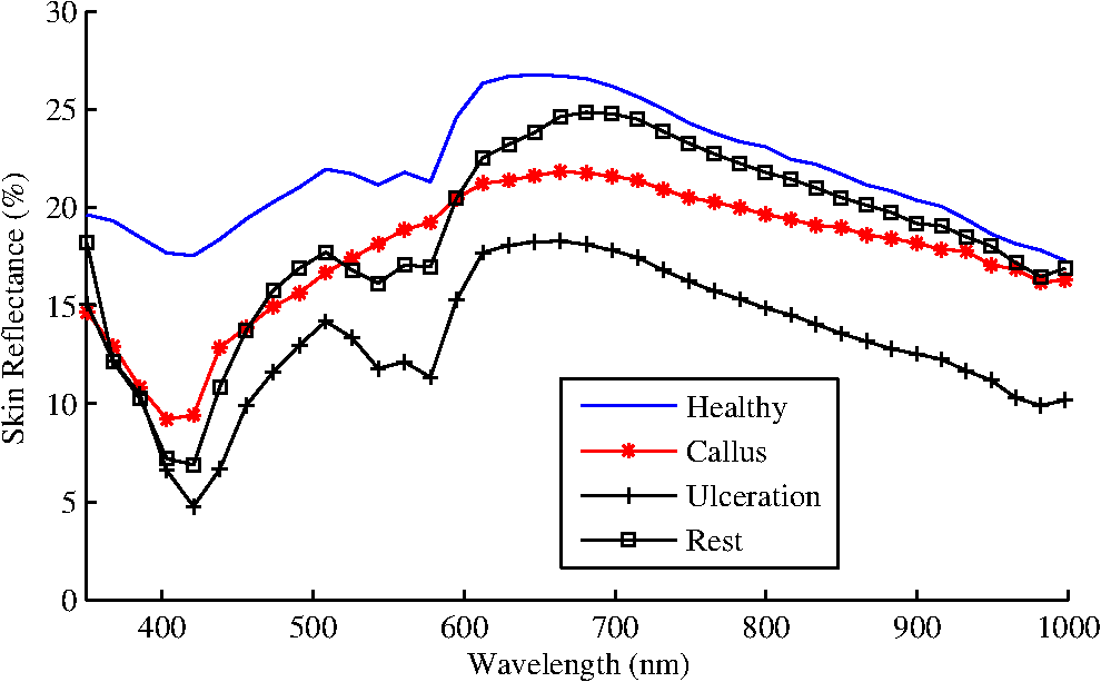
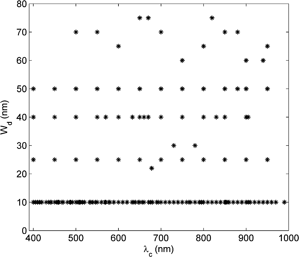
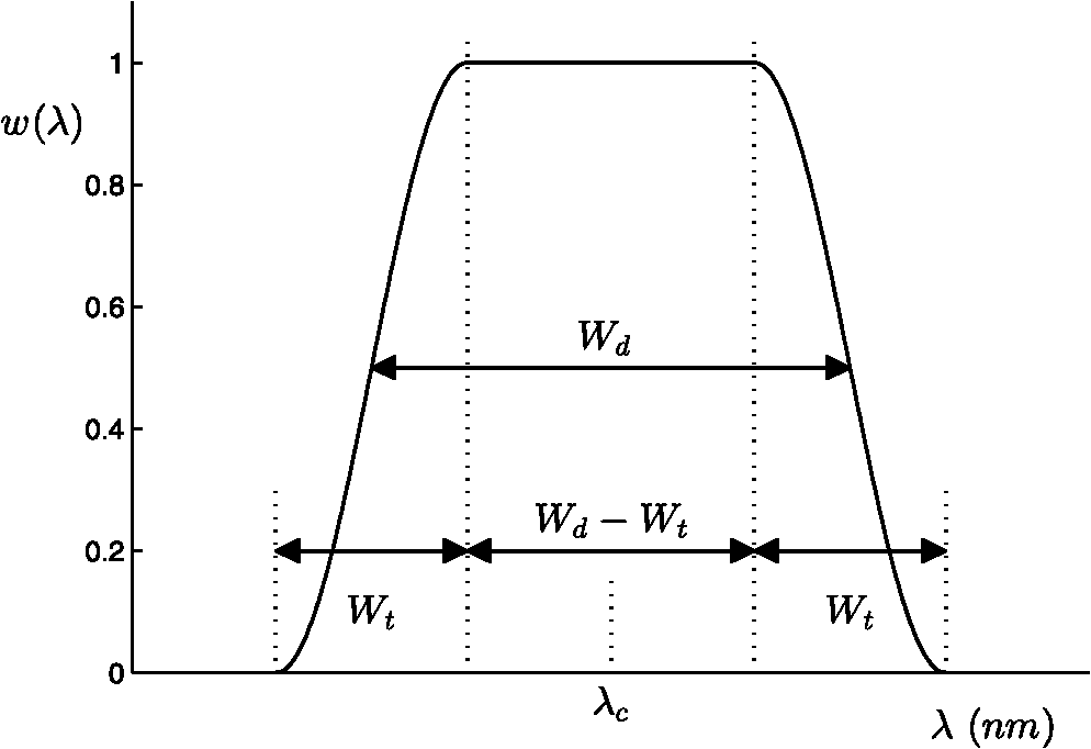
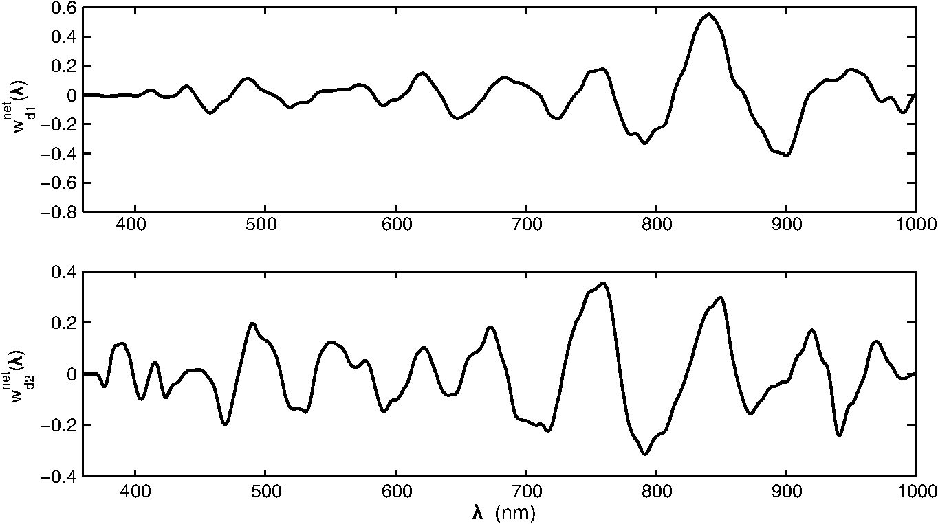
During the measurement, the probe holder was placed on the skin in two directions, which were along the width of the foot and the orthogonal direction. Each ROI was measured two times in each direction. In some cases, when the areas of the ROIs were smaller than $60{\mathrm{mm}}^2$ or on the edge of the foot, only two measurements along the first direction were performed. At least one “Healthy” ROI was measured on each foot of a patient. The final spectra of each ROI was obtained by taking the average of all the four or two measurements.

2.3.

Summary of the Acquired Dataset

Local reflectance measurements were performed on 227 ROIs from 64 patients, among which there were 95 “Healthy,” 55 “Callus,” 38 “Ulcers,” and 39 “Rest.” The “Rest” category bundled several very diverse skin conditions, each of which occurred only infrequently in this study (e.g., 6 necrosis, 5 redness, 3 blister, etc.). In addition, the corresponding areas of some of these ROIs were much smaller than the $60{\mathrm{mm}}^2$ measurement area, so that no pure spectra could be sampled from them. As a consequence, the within-class variation of the data in the “Rest” category was very large. For this reason, the initial statistical analysis, presented in Sec. 3, only focused on the data from the first three classes, which contained 188 of the measured 227 spectra. Examples of the measurements are given in Fig. 3.

Fig. 3

Examples of spectrum from different classes.

3.1.

Methodology for Optical Filter Selection

The functional structure of the statistical analysis is shown in Fig. 4. The database, consisting of the measured and manually classified skin spectra, is fed into a simulator of a large bank of optical filters. The characteristics of these virtual filters match the specifications of real, commercially available bandpass filters. The output data of all simulated filters, as well as the original measured data, is also applied directly to “Classification 1” and “Classification 2” to find the baseline performances, which can help “Filters Selection” to make decisions over the performance of the selected filters. The “Filters Selection” put all the outputs of the simulated filters in a pool to find the (sub-) optimal subset of filters for classifying the measured spectral data. In the subsequent process step “Classification 3”, different classifiers are applied to find the most appropriate one that yields the best performance (i.e., accuracy of classification).

Fig. 4

The functional structure of the data analysis that is applied to find the optimal subset of optical filters.

To make a comparison between the various selections of filters and classifiers, a relevant measure of the performance, such as the error rate (probability of misclassification), is essential. Since overfitting (resulting in a too optimistic estimate of the error rate) can easily occur if the same data is used both for training and for testing, $k$-fold cross validation and/or leave-one-out cross validation¹² is applied to avoid that.

The design of a classifier involves two aspects:¹² (1) selection of the type of classifier and (2) the training of the parameters of the classifiers. The type of classifier (linear, quadratic, Parzen, etc.) defines the structure of the decision function that maps the features to assigned classes. The more complex the mapping is, the more parameters are needed to be estimated to model the mapping, and the more the classifier is susceptible to overfitting. The complexity of a well designed classifier is a compromise between its ability to adapt its decision boundary to the requirements imposed by the statistical properties of the features at hand and its ability to withstand overfitting.

There are two common approaches to reduce complexity, which are feature extraction (FE) and feature selection (FS). The FE approach extracts a set of new features using a simple function that maps the original $N$-dimensional feature space to a lower dimensional space. The features extracted do not have clear physical meanings. The FS approach only selects a subset of existing original features without any mapping. Thus, the FS is the approach that is useful for finding the optimal subset of commercial available optical filters, as presented in Sec. 3.4, whereas the FE will be used in Sec. 3.3 as a reference.

3.2.

Simulation of Optical Filtering

In total, 148 interference bandpass filters were simulated, where the central wavelength ${\lambda }_c$ and the bandwidth $W_d$ of these filters were provided by real filters from two manufacturers: Edmund Optics (York, UK)¹³ and Comar Optics (Cambridgeshire, UK).¹⁴ The ${\lambda }_c$‘s changed from 400 to 1000 nm and the $W_d$‘s varied between 10 and 75 nm. An overview of the parameters of all simulated filters is given in Fig. 5.

Fig. 5

The parameters of the simulated filters. Each point represents a filter.

In addition to the parameters that are specified by the manufacturers, a third parameter $W_t$ was assumed to model the steepness of the filter. $W_t$ is the transition width between zero transmission and maximum transmission, which was set to $W_t=10\mathrm{nm}$. Figure 6 shows the modelled shape of the transfer function $w(\lambda )$, where $W_d$ represents the full width at half maximum and the transition zone is modelled by half a cosine function.

Fig. 6

The modelled filter transfer and the definition of parameters.

The $M_S=188$ spot spectra in the data set were denoted by $R_m(\lambda )$, where $m$ is the ROI number, $m=1,\dots ,M_S$. The $N=148$ filter transfers are denoted by $w_n(\lambda )$. The filter simulation is accomplished by a numerical approximation of:

The filter outputs $z_{nm}$ of each measured area are arranged in $M_S$ $N$-dimensional vectors ${\mathbf{z}}_m$, called feature vectors. The true class for each ROI is available from the diagnosis by experienced clinicians. This yields a labelled training set of $M_S=188$ ROIs, $K$ classes ($K=3$, “Healthy,” “Ulcer,” and “Callus”), and with each spot an associated $N$-dimensional feature vector ($N=148$).

3.3.

Baseline Performance

In order to find a reference for the effects of filter selection, first the performance of classification was assessed with the original measured data and when all filters were used. Direct application of a linear classifier to the full feature vectors ($N=148$) yielded an error rate as high as 70%. Other classifiers yielded likewise performances. The explanation for this behaviour is overfitting. According to a simple rule of thumb,¹⁵ to avoid overfitting in a linear classifier, the number of samples should be at least about five times the number of features ($=\text{number of filters}$). The present case did not fulfill this, and the number of features should be reduced before applying classification. Linear FE was applied to accomplish that.

Linear FE is a linear mapping from ${\mathbb{R}}^N$ to ${\mathbb{R}}^D$ with $D<N$ implemented by a $D\times N$ matrix $\mathbf{W}$:

Two methods are commonly used: linear principal component analysis (PCA) and linear discriminant analysis (LDA). The goal of the PCA is to find the $D$-dimensional linear subspace of ${\mathbf{z}}_m$ that preserves as much variance in the data as possible. Often, $D$ is chosen such that, for instance, 99% of the variance is still in the linear subspace. The PCA projection was always scaled by the mean class standard deviations in this article.

The LDA is a feature reduction method that takes class information into account. If there are $K$ clusters in an $N$-dimensional space, the linear subspace that separates the clusters optimally is at most $D=K-1$ dimension. Hence, for a data set with $K$ classes, the LDA seeks to determine the $K-1$ linear subspace to preserve as much class-discriminatory information as possible: it simultaneously tries to maximize the inter-class distance and to minimize the intra-class distance.

If the original feature space is high-dimensional, and the training set small (as in our case), the LDA must be preceded with PCA to prevent numerical instability.¹² The dimensionality preserved in the preceding PCA should be optimized by cross validation. In our case, the optimal PCA subspace of the 148-D space is a 28-D space, which is further reduced to a 2-D space by LDA. The features extracted as such are illustrated in the scatter diagram in Fig. 7(a). In Fig. 7(b), the figure also shows the scattering of the two most important PCA features. These two features hold 98% of the variance.

Fig. 7

Scatter diagrams in two different feature spaces. (a) Shows the feature space that is obtained by linear discriminant analysis (LDA) [preceded by principal component analysis (PCA)]. (b) Shows the space of PCA features solely.

When the PCA and/or the LDA is applied to the filtered data, as in Eq. (3), each extracted feature is a linear combination of the original filter outputs. Therefore, an extracted feature can be regarded as the output of a single virtual filter. If the elements of $\mathbf{W}$ are denoted by $W_{dn}$, and the $d$‘th element from ${\mathbf{y}}_m$ by $y_{dm}$, then Eq. (3) can be written as:

This effectively implements an optical filter with transfer function:

The net optical filter transfers for the two LDA components are illustrated in Fig. 8.

Fig. 8

The net optical filter transfers for the two LDA components normalized to [0,1].

As shown in Fig. 7, the three classes are discriminated well by the two LDA features, indicating that a simple linear classifier suffices. We verified that by comparing its performance with the ones of a quadratic classifier, a Parzen classifier, a K-nearest neighbor classifier and support vector machine.¹² In all cases, the parameters were optimized using 10-fold cross validation. Besides, 10-fold cross validation was also used to assess the performance. Indeed none of them could out-perform the linear classifier, i.e., they all had similar performances, with a mean error rate 9%. Taking the time consumed for training and classification into consideration, the linear and quadratic classifiers were chosen for the filter selection.

With LDA as the FE and a linear classifier, the error rate of the full set of filtered data was $9\%\pm 1\%$ (obtained with 10-fold cross validation). Exactly the same result was obtained with 28 PCA extracted features directly classified by the linear classifier, instead of indirectly via LDA. Following the same procedure to extract 2 features using LDA (preceeded by PCA), the original measurement data (1127 spectral measurements per ROI) achieved an error rate that was almost the same. The averaged error rate differed $<0.5\%$. We conclude that the simulated filtering did not cause much information loss/gain, and an error rate of $9\%\pm 1\%$ would be used as the baseline, i.e., the reference performance. For illustrative purposes, both of the error rates, from the original measurements (1127-D space) and the data after filtering (148-D space), will be presented in the following sections.

3.4.

Optical Filter Selection

To select filters with the FS techniques, i.e., to find a subset of features corresponding to the full set of filters, two choices have to be made: the search strategy to select candidate subsets, and the search criterion to evaluate these candidates.

Among the available searching strategies,^16,17 the optimal search methods are not applicable, because their searching complexity grows combinatorially. The suboptimal strategies build up the subsets either incrementally (forward), or decrementally (backward). When searching for a relative small subset ($<10$ filters), backward selection is not adequate. Among the three forward strategies, which are sequential forward selection, plus-$l$-take-away-$r$ selection, and sequential floating forward selection (SFFS), the most versatile approach, the SFFS, was chosen.¹⁷

The search criterion can be either a measure of the statistical distance of the class differences in the data, or it can be the estimated error rate of a classifier that is applied to the subset, the so-called wrapper. In this article, one measure, the Mahalanobis distance, and two wrappers, the linear discriminant classifier (LDC) and the quadratic classifier (QDC) are studied. Both wrappers are evaluated with leave-one-out cross validation to avoid overfitting during searching.

To make a comparison between the various selections of filters and classifiers, a relevant measure of the performance, such as the error rate (probability of misclassification), is essential.

The main light-absorbing factors are melanin in the epidermis, and oxy-haemoglobin (${\mathrm{HbO}}_2$) and deoxy-hemoglobin (Hb) in the dermis. The local concentration of each of these factors influences the measured skin spectrum in a specific way. In particular, ${\mathrm{HbO}}_2$ absorption features a strong maximum around 412 nm and additional maxima at 542 and 577 nm, while Hb exhibits peaks at 430 and 555 nm.¹⁸ Thus, these five wavelengths could provide more information about physical parameters, e.g., the epidermal thickness and the oxygen saturation.^19,20

The filter selection was carried out in two different ways: (1) all features/filters had the same eligibility and (2) a constrained selection procedure was done in which center wavelengths, around the five wavelengths listed above, were evaluated and preselected with LDC. Once a subset of filters has been found, the subset must be evaluated empirically. This can be done with any type of classifier. Preliminary research showed that parametric-free classifiers, e.g., Parzen, did not perform better. Hence, we selected LDC and QDC once again for empirical evaluation. 10-fold cross validation was used to assess the error rate.

3.4.1.

Filter selection without preselection

The evaluation results are shown in Fig. 9. The SFFS strategy may return with a smaller number of features than the number that is requested when it detects that addition of features does not improve the search criterion. Six features were returned when using LDC as the searching criterion, while four features were returned when using QDC as the searching criterion. When comparing the performances, the observations are:

• (1) With a set of appropriate chosen filters, the performance of all criteria compares well with the baseline performance.

• (2) The performance associated with the Mahalanobis search criterion converges slower than the other criteria. Apparently, the Mahalanobis criterion finds less strong features.

• (3) The Mahalanobis search criterion, evaluated with QDC, yields the lowest error rate at five filters.

• (4) The performances of LDC and QDC search criteria peak at three and four filters, respectively. Adding more filters does not improve the performance significantly, or could even worsen the performance.

• (5) For a smaller number of filters, the QDC classifier generally performs better, indicating that the classes are better separated by quadratic decision functions than linear ones.

Fig. 9

Classification accuracy for sequential floating forward selection (SFFS) with different criterions, linear discriminant classifier (LDC) as classifier (solid lines) and quadratic classifier (QDC) as classifier (dashed lines) for empirical evaluation. The gray color bands represent baseline error rate achieved with features extracted from LDA with LDC as classifier with the original spectra data (1127-D), while the red colour bands represent the baseline achieved with the features extracted from LDA with LDC as classifier with the spectra data after filtering (148-D).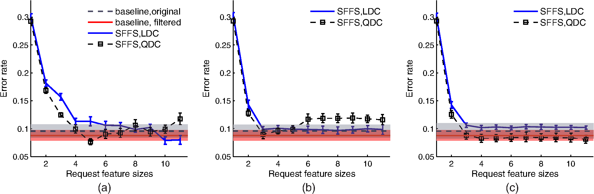

The found subsets are given in Table 1. As can be seen in Fig. 10, each subset seeks information in the range of 550 to 600 nm, and the LDA features are formed by differentiating filter outputs. This results in a large impact on noise sensitivity, to be discussed in Sec. 4. The Mahalanobis distance seeks additional information in a range around 400 nm. The LDC and the QDC both find information in the range around 650 nm useful.

Table 1

The best subsets of filters (unconstrained search). Each filter is defined by the parameter set “λc (Wd)” given in nm.

Search criterion	${\text{Filter}}_1$	${\text{Filter}}_2$	${\text{Filter}}_3$	${\text{Filter}}_4$	${\text{Filter}}_5$
Mahalanobis	570 (10)	570 (40)	589 (10)	415 (10)	400 (40)
Linear discriminant classifier (LDC)	570 (10)	550 (25)	647 (10)	—	—
Quadratic classifier (QDC)	632.8 (40)	570 (10)	550 (25)	690 (10)	—

Fig. 10

The net optical filter transfers that produces the two LDA components of the 3-class problem. These transfers, normalized to [0,1], correspond to three feature subsets as given in Table 1.

3.4.2.

Filter Selection with pre-selection

In addition to the five filters predefined, this constrained FS procedure selected up to six other filters from the rest pool. The results are shown in Fig. 11. Ten-fold cross validation was used to assess the error rate.

Fig. 11

Classification accuracy for the SFFS with different criteria, the LDC as classifier (solid lines) and the QDC as classifier (dashed lines). The feature selection started from 5 predetermined filters.

Again, the QDC as an evaluation classifier often performed better than the LDC. The best results were obtained when QDC was used for the selection criterion as well as for empirical evaluation [Fig. 11(c)]. With 10 features, the number of ulcer ROIs (i.e., 38) is somewhat less than four times the dimension, whereas it should be at least five times to prevent overfitting, according to the rule of thumb.¹⁵ Apparently, it paid off to allow quadratic decision boundaries (rather than linear), although the additional parameters for the quadratic boundaries resulted in some performance loss due to overfitting.

The QDC in Fig. 11(c) obtains a minimum with seven features. The performance improvement with the additional three features is not statistically significant. The filter parameters (${\lambda }_c$ and $W_d$, in nm) that are associated with these features are, where the first five are the predefined filters: 540 (10), 430 (10), 400 (50), 580 (10), 550 (40), 730 (30), 410 (10).

3.4.3.

The “Rest” class

Up to now, the ROIs in the “Rest” category were ignored. As said before, the “Rest” consisted of a number of different subclasses that were often formed by tiny spots closely surrounded by healthy skin, callus, or ulcer. To see how the rest class behaves, Fig. 12 shows a scatter diagram of all spots in the posterior probability space that is spanned by $P(\text{callus}|\mathbf{y})$ and $P(\text{ulcer}|\mathbf{y})$. Here, $\mathbf{y}$ represented the 7-D feature vector that was tabulated in Sec. 3.4.2.

Fig. 12

The scattering of the data set in the posterior probability space and the decision boundaries, under assumption of equal prior probabilities and equal cost of misclassification.

The posterior probabilities were calculated under the assumption of class dependent, Gaussian likelihood functions, as the base of the quadratic classifier.¹² The quadratic decision boundaries in the feature space are mapped to linear boundaries in the probability space.

When “Callus” and “Ulcer,” with or without “Rest,” were conflated to one class “Unhealthy,” the estimated performances of the subsets selected are listed in Table 2. When “Rest” is included, the sensitivities dropped from $\sim 96\%$ to $\sim 90\%$ and AUC decreased with 0 to 0.2, while the specificities all raised $\sim 1\%$. Based on the table, all subsets selected with different criteria did similar and sufficient good work in classification. It is still hard to make a choice among these selected subsets.

Table 2

Performance of the filters selected.a

Searching criterion	No. of filters	No “Rest” class			With “Rest” class
		Sensb	Spec	AUCc	Sens	Spec	AUC
Mahalanobis	5	95%	96%	0.98	91%	97%	0.97
LDC	3	95%	92%	0.97	93%	93%	0.97
QDC	4	97%	94%	0.96	91%	95%	0.96
QDCd	7	97%	96%	0.99	89%	98%	0.97

^aResults obtained with 10-fold cross validation.

^bSens = Sensitivity and Spec = Specificity.

^cAUC = Area under Receiver operating characteristic curve.

^dWith preselection.

3.5.

Discussion of the Optical Filters Selection

The four subsets of filters that are presented all operate in the wavelength range around 550 nm. Two selections also operate in the vicinity of 400 nm. These ranges are all in the biomedical window. None of the selections operate above 750 nm. There is some resemblance between the filters that are based on the LDC and the QDC criteria, but apart from that, the different solutions do not have much intersection. The selection of filters is not very critical as different subsets perform equally well. In all subsets, the QDC outperforms the LDC. This suggests that the dispersion of the measurement data is class dependent. For class independent dispersion, the QDC degenerates into LDC. Since the dispersion of data is caused by the skin properties and not by measurement noise, a class dependent dispersion makes sense.

The “Rest” class is not included in the classifier design as yet. Figure 12 shows that the “Rest” ROIs are either situated at the three clusters that correspond with “Healthy,” “Ulcer,” and “Callus,” or situated in-between pairs of those clusters. The explanation is that the areas of “Rest” ROIs are smaller than the measurement area. As a consequence, the measured spectra represent a mixed response from the “Rest” ROIs and the surrounding areas belonging to one or several other classes. For instance, all six measurements for necrosis points in the “Rest” category were classified as “Ulcer,” as shown in Fig. 12. On the other hand, three out of five measurements from redness were classified as “Healthy,” one measurement was classified as “Callus” and the other as “Ulcer.”. The same “mixed area” effect occurs in fact also for several ROIs labelled to the other classes. This also explains the phenomenon that the specificity rose when the “Rest” class was added, as shown in Table 2.

For a real spectral camera, the pixel size will be much smaller than $60{\mathrm{mm}}^2$, the spectrometer measurement area, and the problem will not occur. However, the classifier needs retraining then, because the rest class is not included as yet.

4.1.

Monte Carlo Analysis

The stability analysis was carried out by means of a Monte Carlo analysis applied to three different configurations of filter subsets and classifiers:

Configuration 1 was chosen since its performance and its parsimony were the best that could be obtained. Configuration 2 was added to see whether the quadratic classifier was less stable than a linear classifier. Configuration 3 was chosen to see whether a large number of filters (a less parsimonious design) would degrade the stability.

The Monte Carlo stability analysis was done as follows. After random sampling of the parameter of a configuration, the error rate of that configuration was estimated using 10-fold cross validation. This was repeated 100 times, and the average over these 100 estimates are shown in Fig. 13. The procedure is repeated for four parameters: the center wavelengths ${\lambda }_c$, the bandwidths $W_d$, the widths $W_t$ of the transition band, and the maximum expected number of electrons. The latter parameter determines the signal-to-noise ratio (SNR) of the system.

Fig. 13

The influence of tolerances of filter parameters and the influence of shot noise. The performance is given in classification error rate. “UNC” and “CON” present unconstrained and constrained selection, respectively.

The manufacturers specify tolerance regions for ${\lambda }_c$’s and $W_d$’s. For different $W_d$’s and different coating approaches, the tolerances may be different. For example, when $W_d=50\mathrm{nm}$, the tolerance is $\pm 15\mathrm{nm}$ if traditionally coated, and $\pm 5\mathrm{nm}$ if hard coated. When $W_d=10\mathrm{nm}$ the tolerance is $\pm 2\mathrm{nm}$. When $W_d=25$ or 30 nm the tolerance is $\pm 3\mathrm{nm}$.^13,14

Note that the transmission coefficient of the spectral filters, which varies from 30% to 90% for the types of filters considered here,^13,14 need not be included in the stability analysis. This is because it can be assumed that the response of a given imaging system (including light source, image sensor, lens, and the filters) is calibrated for each filter using e.g., a white reference standard, and that it remains calibrated during the measurements. However, low transmission coefficients may influence the SNR.

The SNR of the imaging system may be another important aspect that affects the classification stability. The random count of electrons, which are generated at the image sensor during the exposure time, defines the image output and decides the shot noise.²¹ The probability of this count obeys Poisson distribution, and according to that property, the expectation of the count equals its variance, $E[\text{count}]=\mathrm{Var}[\text{count}]=\mathrm{\Phi }$. Then, the SNR can be expressed as

Each parameter was submitted to the Monte Carlo analysis by random sampling according to distributions of the parameters that modelled the tolerances:

Then, all features are transformed to the expected electron count using the factor $K=\mathrm{\Phi }/y_{\max }$. According to Eq. (6), Gaussian noise was added to each feature with a variance that equals $\mathrm{\Phi }$. Finally, the features were back-transformed by a factor $1/K$.

Figure 13 shows the results of the Monte Carlo analysis. The estimated errors all had standard deviations around 1%.

4.2.

Discussion of Stability Analysis

When comparing the results with respect to the three configurations of filter subsets and classifiers in Fig. 13, no substantial differences in behavior can be observed. The linear classifier is not more stable than the quadratic classifier, and using only four filters instead of seven does not contribute much to stability either.

The shape of the filter transfer function is modelled by the bandwidth $W_d$ and by the width $W_t$ of the transition band. Figures 13(a) and 13(b) show that the classification performance is not sensitive to changes of these parameters. The results suggest that such an assumption is not very critical: with extreme values of $W_t$ the modelled transfer functions vary between a rectangular window and a very smooth cosine window, but the performances are not affected.

Figure 13(c) shows that shifts of the center wavelengths of the filters may reduce the performance. If an increase of error rate of 1% is permitted (about equal to the uncertainty of the estimated error rate), the standard deviation of the shifts should not be more than about 4 nm. This requirement is equal to the specification of the low-cost commercial filters, so that it can be fulfilled easily when designing the SI system.

The most critical parameter appears to be the maximum expected electron count, $\mathrm{\Phi }$. The explanation is that the differences between the outputs of filters are important for classifiers to discriminate different classes (as illustrated in Fig. 10). This may drastically reduce the SNR, i.e., even a small amount of noise has a large impact on the difference. Figure 13(d) indicates that $\mathrm{\Phi }$ should be above ${10}^6$ to avoid a performance decline due to quantum limitations. In a hyperspectral camera, such a high density of electrons can be realized by (a) powerful illumination, (b) large exposure time, (c) large aperture of the optics, (d) large pixel size, (e) detective quantum efficiency close to 100%, and (f) transmission of the filters close to 100%. However, the ultimate limitation is defined by the saturation level of the image sensor. For a high-quality industrial camera module with 4 Mp resolution, a typical saturation level is $4\times {10}^4$. The figure shows that at that level the increase of error rate can be as high as 2%; the subset of seven filters a little higher than the one with four filters. If such a loss of performance cannot be tolerated, the effective electron count can be increased by using a sensor with a large pixel size, and by summing over neighboring pixels or subsequent frames. The price to pay for an increased pixel SNR is increased system costs, and reduction of spatial and temporal resolution.