Real-time monitoring of changes in plasma membrane potential via imaging of fluorescence resonance energy transfer at individual cell resolution in suspension

Tzachi Sabati; Bat-Sheva Galmidi; Alon Korngreen; Naomi Zurgil; Mordechai Deutsch

doi:10.1117/1.JBO.18.12.126010

16 December 2013 Real-time monitoring of changes in plasma membrane potential via imaging of fluorescence resonance energy transfer at individual cell resolution in suspension

Tzachi Sabati, Bat-Sheva Galmidi, Alon Korngreen, Naomi Zurgil, Mordechai Deutsch

Author Affiliations +

Journal of Biomedical Optics, Vol. 18, Issue 12, 126010 (December 2013). https://doi.org/10.1117/1.JBO.18.12.126010

Abstract

A method for monitoring heterogeneity in changes of plasma membrane potential (PMP) at an individual cell resolution while in suspension, utilizing a simple and low-cost wide-field illumination arrangement, is presented. The method is modeled via HEK-293 cell line in suspension, double stained with coumarin and oxonol (donor and acceptor), which were loaded into an array of nanoliter wells, each designed to preserve the individuality of the nontethered cell it holds during vigorous biomanipulation. Depolarization of PMP was induced by high K + solution, reducing the proximity between the membrane fluorophores and subsequently reducing the efficiency (E% ) of resonance energy transfer between them. Spatial plots of E% were produced from both images of fluorescence intensity and polarization. The spatial resolution of E% plots seem to be higher, and their contrast greater, when calculated from the polarization, rather than from the intensity of the fluorescence.

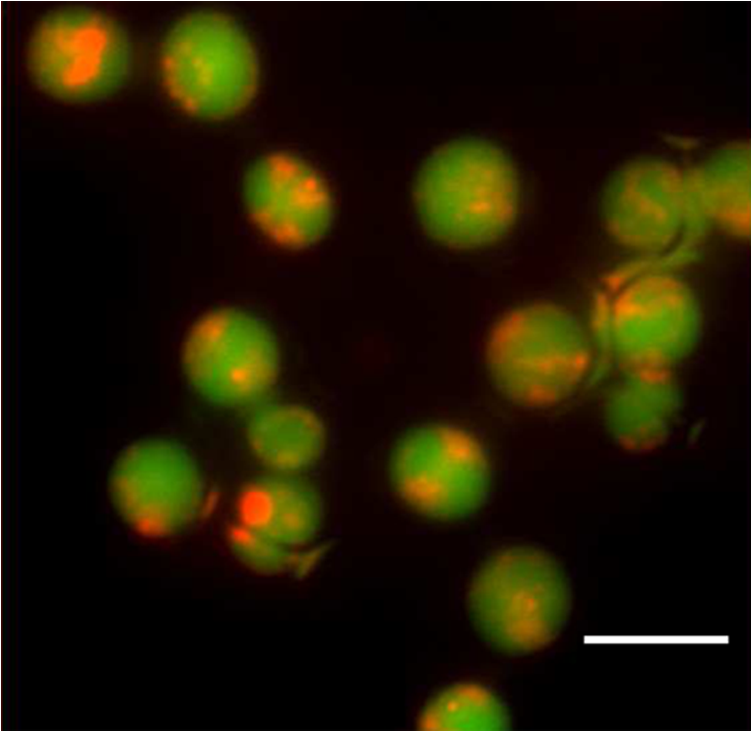
1. Introduction

Ion channels constitute a class of integral membrane proteins that regulate the flow of ions across the membranes of all cells. The main role of ion channels is in the membrane of electrically excitable cells, such as neurons, cardiac myocytes, and skeletal muscle fiber. In addition, they are key components in a wide variety of biological processes that involve rapid changes in cells, including epithelial transport of nutrients and ions, T-cell activation and pancreatic beta-cell insulin release. Ion channels can be found in virtually every cell type throughout the body and have been implicated in the pathogenesis of multiple diseases.¹ In recent years, ion channel targets are of growing interest for drug discovery and development.²^–⁶

Functional evaluation of ion channels requires a sensitive, simple assay and instrumentation that will report ion channel activity in living cells. Membrane potential assays are used for screening many types of ion channels, since the change in the membrane potential reflects the activity of the channel of interest.²

The gold standard assay for assessing functional activity of ion channels in mammalian cells is patch clamp electrophysiology, introduced by Neher and Sakmann.⁷ Recently, major advances have been made in the development of automated electrophysiological platforms to increase capacity for such cell-based methods.³^,⁸

Optical methods introduced by Cohen⁹ allow investigation of large populations (over $10^{4}$ cells) on a single cell basis. Several fluorescent dyes optimized to measure membrane potential changes with high sensitivity are on the market,¹⁰^,¹¹ some of which have been recently adapted to high throughput screening (HTS) (Ref. 12).

González and Tsien¹³ developed a method to estimate membrane potential based on the Forster type singlet–singlet resonance energy transfer between appropriately selected fluorescence donor and acceptor couples, where the donor is located on the extracellular surface of the plasma membrane, and energy is transferred to the membrane-permeable negatively charged acceptor which translocates across the membrane due to changes in membrane potential. Gonzales and Tsien¹³ monitored membrane voltage via fluorescence intensity (FI) based fluorescence resonance energy transfer (FRET) measurement.

Based on Damjanovich et al.’s approach,¹⁴ imaging of FRET efficiency ( $E %$ ) via fluorescence polarization (FP) has already been demonstrated in 2002.¹⁵^,¹⁶ However, in these studies, calculation of $E %$ was not performed on the same individual cell, but was rather based on the comparison between the FP of a single cell double-stained with donor–acceptor and a population based average FP of cells stained only with the donor. Others used FP as an indication for FRET rather than for the calculation of $E %$ -images. This includes occurrences of FRET either between different molecules (hetero-FRET) or between the same type of molecule (homo-FRET).¹⁷^–²¹ Though not among individual cells in suspension, these studies, as many others, have examined FRET in various biological models, utilizing sophisticated, costly, frequency-based or time-domain-based fluorescence lifetime (FLT) imagers.

The present study, utilizing a low-cost, wide-field illumination arrangement, focuses on monitoring changes of plasma membrane potential (PMP) at an individual cell resolution in suspension, which may potentially enable exploration of nonadherent cell heterogeneity with regard to changes in their PMP. This approach is realized by the use of picoliter well (picowell) arrays,²² each of which can hold a cell without tethering. Measurement of FI and polarization was performed on the same individual cells, before and after the induction of membrane electrical depolarization, yielding cellular spatial distribution of $E %$ in arrayed single cells.

1.1.

Mechanism and Theory

Monitoring of changes in PMP by measurement of $E %$ was demonstrated on individual HEK-293 cells which were double stained with coumarin (CC2-DMPE, donor) and oxonol (DiSBAC2(3), acceptor). The former fluorophore is a membrane-bound phospholipid, which binds only to the exterior of the cell membrane. The latter is a mobile, negatively charged hydrophobic molecule, which will bind to either side of the plasma membrane in response to changes in the PMP.

At resting PMP, oxonol binds to the outer side of the membrane, near the coumarin. However, following biological activation, membrane potential decreases, which is manifested by electrical depolarization of the plasma membrane, and results in elevation in negative charge concentration at the outer side of the membrane. Finally, this induces the translocation of the negatively charged acceptor (oxonol) onto the positively charged inner layer of the plasma membrane, reducing its proximity to the donor. In other words, the smaller the membrane potential, the more the oxonol tends to move toward the interior layer of the membrane, increasing its distance from the donor coumarin.²³ On the other hand, the greater the distance, $r$ , between the donor and the acceptor, the lower the chance for dipole-dipole interaction to occur between the couple. Consequently, the efficiency ( $E %$ ) of FRET is reduced following Förster:²⁴

E = \frac{R_{0}^{6}}{R_{0}^{6} + r^{6}},

where

R_{0}

is the distance at which the average chance for an excited donor relaxation to occur via either emission or FRET is equal. Next, since both options (emission and FRET) of evacuating the excited level of the donor are active, donor FLT-

τ_{F}

(of the excited state in the absence of acceptor) is shortened, consequently increasing its FP. The transition from FI to FP based

E %

calculation has been discussed elsewhere.¹⁵ Very briefly, Perrin’s equation teaches that²⁵

Eq. (1)

\frac{1}{p} - \frac{1}{3} = (\frac{1}{p_{0}} - \frac{1}{3}) \cdot (1 - \frac{τ}{τ_{r}}),

where

p

is the measured FP,

τ

is the excited state lifetime,

τ_{r} = η V / R T

is the rotational correlation time of a spherical-like molecule suspended in a homogeneous solution in which

η

is the solvent viscosity,

V

is the Molar volume of the fluorophore,

R

is the gas constant, and

T

is the absolute temperature and

p_{0}

is the FP at

(T / η) \to 0

. From Perrin’s equation one can express the donor’s de-excitation lifetime in the absence (

τ_{D}

) and in the presence (

τ_{D}^{A}

) of the acceptor, as follows:

Eq. (2)

τ_{D} = τ_{R} (\frac{1 / p_{D} - 1 / p_{0}}{1 / p_{0} - 1 / 3}),

Eq. (3)

τ_{D}^{A} = τ_{R} (\frac{1 / p_{D}^{A} - 1 / p_{0}}{1 / p_{0} - 1 / 3}),

where

p_{D}

and

p_{D}^{A}

are the FP of the donor in the absence and in the presence of the acceptor, respectively. Next, substituting Eqs. (2) and (3) into the well-known relation

E = 1 - τ_{D}^{A} / τ_{D}

yields:

Eq. (4)

E (p_{D}, p_{D, 0}) = \frac{p_{0, D} (p_{D}^{A} - p_{D})}{p_{D}^{A} (p_{0, D} - p_{D})},

where

p_{0, D}

is the donor

p_{0}

.

p_{D}

and

p_{D}^{A}

are the double stained cell pre- and postactivation values, respectively, which in the present study is denoted by

p^{D A}

and

p^{D \to A}

[see Eq. (7)], where

D A

and

D \to A

indicate the corresponding donor (CC2-DMPE) to acceptor [

{DiSBAC}_{2} (3)

] proximity.

Even though Eq. (1) holds true for small ( $< 300 Da$ ), spherical-like fluorophores immersed in a homogeneous media,²⁶ it firmly reflects the reciprocal “rule of thumb” between the measured FP of a fluorophore and its FLT, and hence its use in the consequent formulas presented above.

2. Experimental

2.1.

Materials

Voltage Sensor Probe Set CC2-DMPE (coumarin), ${DiSBAC}_{2} (3)$ (oxonol), and Pluronic® F-127 were purchased from Invitrogen Corporation (Carlsbad, California). VSP-1 medium solution contained 160 mM NaCl, 4.5 mM KCl, 2 mM ${CaCl}_{2}$ , 1 mM ${MgCl}_{2}$ , 10 mM glucose, 10 mM 2-[4-(2-hydroxyethyl)piperazin-1-yl]ethanesulfonic acid (HEPES), pH 7.4. VSP-2 solution provided a high $K^{+}$ concentration, containing 164.5 mM KCl, 2 mM ${CaCl}_{2}$ , 1 mM ${MgCl}_{2}$ , 10 mM glucose, 10 mM HEPES, pH 7.4.

Tetramethylrhodamine methyl ester (TMRM) was obtained from Sigma–Aldrich (St. Louis, Missouri). Fluorescein diacetate (FDA) was purchased from Sigma-Riedel-de-Haen (Hanover, Germany). Hoechst 33342 trihydrochloride, trihydrate, was purchased from Invitrogen-Molecular Probes (Carlsbad, California).

2.2.

LiveCell™ Array (LCA)

The LCA is a configured micro-fluidic based microscope-slide device²² containing a 2.5 μl cell chamber (see Fig. 1). The upper entrance of the cell chamber ( $φ 2$ mm cylindrical aperture) is level with the bottom of an open micro-conduit. The bottom of the cell chamber (0.7-mm deep) comprises about 7800 hexagonal glass pico-liter wells (picowells), 20 μm pitched, $\sim 7 - μ m$ deep. The picowell walls have extremely sharp edges ( $< 0.1 - μ m$ wide) designed to gently direct the cells to settle in the picowells, rather than in the space between them. Hence, cell loading is efficient, enabling the use of extremely low sample sizes. Within the array, nonadherent cells are individually maintained without tethering, each in its own picowell, enabling long term measurement during various vigorous biomanipulations, such as medium exchange, multiple staining, washing, drug treatment, and more.

Fig. 1

The LiveCell™ array and HEK-293 cells in picowells. Upper panel: Top view of the LCA ( $1 \times 3 in$ .). The 2.5 μl cylindrical cell chamber (1) is engraved into the LCA’s plastic body (2) and its bottom made of glass picowells (small milky region inside the chamber) and they are 20 μm pitched (white scale bar). The cover slip (3) can be dragged left and right via its handles (4) to enable loading of cells into the cell chamber and presentation of liquids into the entrance of the open conduit (see Fig. 2). Lower panel: An overlapping image of the fluorescence and bright field images of individual HEK-293 cells in their picowells, as they appear at the bottom of the cell chamber, following double staining with Hoechst 33342 and TMRM.

The high optical quality of the picowells allows the performance of high content image analysis of the cells maintained during manipulation, at individual cell resolution. The entire arrangement—conduit and cell chamber—is secured by a cover slip (170-μm thick). For loading of cells, the chamber entrance is uncovered by dragging the cover slip leftward. Cell suspension is then introduced into the chamber, after which its entrance is re-covered, to allow capillary flow of relevant solution in the gap between the cover slip and the conduit.

2.3.

Preparation of HEK-293 Cell Suspension

A HEK-293 cell line was grown in a humidified atmosphere containing 5% ${CO}_{2}$ , in RPMI 1640 medium (Biological Industries, Israel), supplemented with 10% (v/v) heat inactivated fetal calf serum (Biological Industries, Israel), 2 mM l-glutamine, $50 U / ml$ penicillin, and $100 mg / ml$ streptomycin. The cells were harvested by incubation for 3 min in room temperature with 0.25% Trypsin–EDTA solution B (Biological Industries, Israel) and washed by centrifugation for 5 min at room temperature with VSP-1.

Single HEK-293 cells in suspension, each in its own picoliter well, were viable, as indicated by their mitochondrial membrane potential and by their ability to hydrolyze FDA and to retain fluorescein (Fig. 2).

Fig. 2

Viability of single HEK-293 cells within LCA. Overlapping fluorescence images of HEK-293 cells double stained with TMRM and FDA. Scale bar: 20 μm.

2.4.

Cell Staining CC2-DMPE (Coumarin), DiSBAC₂ (3) (Oxonol)

For cell staining with voltage sensor probes set, $\sim 2.5 \cdot 10^{6}$ cells were incubated at 25°C for 30 min within 0.5 ml VSP-1 solution that contains 25 μM CC2-DMPE and $100 mg / ml$ Pluronic F-127. The cells were washed once by centrifugation, free of CC2-DMPE, for 5 min at 25°C, and then washed again by centrifugation for 5 min at 25°C with VSP-1, and the supernatant was removed. Cells were re-labeled by ${DiSBAC}_{2} (3)$ and the sample was maintained for 30 min at 25°C. The final concentration of ${DiSBAC}_{2} (3)$ was 5 μM. The cells were washed once by centrifugation, free of ${DiSBAC}_{2} (3)$ , for 5 min at 25°C, and then washed again by centrifugation for 5 min at 25°C with VSP-1, and the supernatant was removed. Finally, the membrane depolarizing solution VSP-2 was added to the cells while in LCA.

Simultaneous measurements of mitochondrial membrane potential and esterase activity in the same cells were accomplished by first staining with 200 nm TMRM (emission wavelength 580 nm) for 15 min at 37°C, 5% ${CO}_{2}$ , followed by washing with PBS and addition of 1.2 μM FDA (emission wavelength 530 nm). For staining of cell nucleus, cells were incubated with 20 μl Hoechst 33342 dye ( $5 μ g / ml$ ) in PBS for 30 min at RT in the dark.

2.5.

Cell Loading and Solution Presentation into the LCA

Following sliding of the LCA cover slip and exposure of its cell chamber, 7.5 μl of the double-labeled HEK-293 cells ( $1.5 - 2 \times 10^{6} cells / ml$ , suspended in VSP-1) were poured into it and left for 7–10 min to sediment onto the picowell-padded-bottom of the chamber. Next, 5 μl of the (upper) supernatant was removed, leaving a 0.15 mm gap between the cover slip and the conduit, thus allowing closure of the cover slip without getting it wet. To enable optical observation, this gap was filled with 5 μl VSP-1 solution, simply by introducing the aliquot on top of the front basin, against the space between the open conduit and cover slip. The introduced medium travels between the two along the chamber opening by means of capillary forces created between the open conduit plane and the cover slip above it.

Finally, to depolarize the cell membrane of cells in the LCA, the solution VSP-2 was introduced following the procedure described above. However, to ensure complete exchange of VSP-1 by VSP-2, 3 to 5 times the chamber volume ( $2.5 μ l \times 3$ or 5) was introduced, whereby the VSP-2 reached the cell layer on the chamber bottom, replacing the previous VSP-1 leftovers via local turbulence created near by the chamber edges, as well as diffusion. Cells are now suspended in VSP-2 ready for further observation.

Procedures and related performances in regard to cell loading into and solution exchange within the LCA are demonstrated in real time in three movie clips.²⁷ Briefly, Parts 1 and 2 are macro-views of liquid flow and liquid exchange within the LCA chamber, respectively. Part 3 demonstrates cell loading and solution exchange within the LCA.

2.6.

Optical Observations

2.6.1.

Measurement system

Fluorescent labeled cells were imaged using an epi-fluorescence microscope (BX61, Olympus, Japan), with a $20 \times 0.4 NA$ LCPlanFl objective (Olympus, Japan) and Hg lamp (Olympus, Japan). Images were obtained by the photometric ${CoolSNAP}_{H Q}$ monochrome charge-coupled device (CCD) camera with a $1392 \times 1040$ imaging array and $6.45 \times 6.45 μm$ pixels (Roper Scientific, Inc., Trenton, New Jersey). The donor fluorescent agent CC2-DMPE was detected using coumarin filter cube (excitation 405 nm, emission 460 nm, Chroma Technology Corporation, Brattleboro, Vermont). The control of the microscope, filter and polarizer wheels, data acquisition and processing, including FP calculation, were performed using in-house macros written for the Image-Pro Plus (IPP) software (Media Cybernetics, Inc., Rockville, Maryland).

2.6.2.

Preparation of microscope for FP measurement

The microscope was modified to enable FP measurement. An excitation polarizer (Edmond Industrial Optics, Barrington, New Jersey) was inserted across the excitation beam to determine its polarization. On the emission side an analyzing polarizer couple was set perpendicularly ( $⊥$ ) and in parallel ( $‖$ ) with respect to the excitation polarization plane. Practically, the analyzing polarizers were installed in a motorized filter wheel (Olympus, Japan), which allowed totally computer-controlled FP measurement.

The adjustment of fluorimeter for FP measurement might be complex and of epifluorescence microscopes in particular. In short, the procedure is a three step process. First, the excitation polarizer and the emission analyzing polarizers are aligned with respect to the microscope optical axis. The use of the removable microscope built-in polarizers (for differential interference contrast) as references, eases the alignment. Polarization of the excitation beam, measured at the objective front focal plane, was found to be $> 0.987$ . Second, polarization calibration by predetermined transmitted (Halogen) light is performed. A testing polarizer (TP) is attached to a controlled rotating table, which is inserted between the condenser and the microscope objective. Via the rotating table, the light polarization is exactly determined by meticulously setting the angle ( $φ$ ) between the plane of polarization of the TP and that of the microscope emission orthogonal ( $S$ ) analyzing polarizer. Under this setting, the transmitted light polarization $P$ equals cos $2 φ$ . Third, micro- versus macro-FP measurements of the same fluorescent solutions are performed (fluorescein in different concentration of glycerol in water). FP values of these solutions are determined by macroscopic, $L$ or $T$ shape, spectrofluorimeter, which is considered an ultimate optical arrangement for FP measurements. Regarding the last two steps, it is recommended to use polarization values (standards) within the relevant dynamic range, say 0.100 to 0.400. This is achieved by setting the TP angle in the range $42 \deg - 34 \deg$ and the glycerol concentrations (V/V) in the range 60 to 80%.

The FP images obtained with standards (either of transmitted light or of fluorescent solutions) were highly homogeneous. The CV of FP values of either the same pixel or between pixels in the image was $< 0.8 %$ . For further details see Ref. 16.

2.6.3.

Acquisition of images of FP from FP components

For each field of observation, four images of cells in the field were acquired: ${FI}_{‖}^{D A}$ , ${FI}_{⊥}^{D A}$ , ${FI}_{‖}^{D \to A}$ and ${FI}_{⊥}^{D \to A}$ , the polarization intensity components of the preactivated (having standard PMP) and the postactivated cells, respectively.

Next, images were converted from 12-bit gray scale to a floating point format, in order to perform the appropriate calculations. For each image, the background was established by plotting the FI along the scale line (profile line) in the image, when at a distance from the fluorescing cells. This constant background (i.e., the scattered light, camera dark current, and the uniform weak fluorescence background—in all, less than one percent of the cell fluorescence signal) was subtracted from the acquired image. The image underwent segmentation using the standard IPP procedure, allowing the creation of a binary mask, i.e., assigning to all cells an FI unit value, and to areas outside the cells (that not recognized in the segmentation) a null value. The masks were calculated for each of the abovementioned images and were separately applied to those acquired via the parallel and perpendicular polarizers.

This procedure resulted in an image of cells with proper fluorescence intensities and a uniformly zero background between cells.

2.6.4.

Formation of FP and FI images

To form an FP image (map) out of the acquired FI polarization components, a couple of corresponding ${FI}_{‖}$ and ${FI}_{⊥}$ images were synchronized on a pixel basis [matching between corresponding pixels $(i, j)$ of the two FI images] to allow accurate spatial FP calculation.

The algorithm used for registration was “direct alignment method” of Image-Pro Plus software (Media Cybernetics Inc., Rockville, Maryland).

Eventually, a calculated filtered FP ( ${FP}_{f}$ ) image was obtained by processing the filtered ${FI}_{‖}$ and ${FI}_{⊥}$ images according to the following formula:

Eq. (5)

{FP}_{f} (i, j) = \frac{{FI}_{‖} (i, j) - M {FI}_{⊥} (i, j)}{{FI}_{‖} (i, j) + M {FI}_{⊥} (i, j)} .

The indices (

i

,

j

) denote the location of the pixel in a row

i

and a column

j

on the image plane. Here,

M

is the microscope correction factor that compensates for the distortion of FP measurement due to the microscope objective numerical aperture and optical pass.¹⁵^,²⁸ For all intents and purposes,

M = {FI}_{∥}^{NPL} / {FI}_{⊥}^{NPL}

, where the intensities of the polarization components are of a nonpolarized light (NPL) source (i.e., the microscope halogen lamp). Obviously, in an optically nondistorted system,

M = 1

. However, in our microscope

M

was found to equal 0.87.

Finally, FP image smoothing was performed with a Median filter ( $7 \times 7$ , 1 pass). From the FP images of single-labeled cells, the mean cellular FP was calculated, while the FP images of double-labeled cells served as the basis for $E %$ imaging, as described below.

Images of FI were obtained similarly according to the formula:

Eq. (6)

{FI}_{f} (i, j) = {FI}_{∥} (i, j) + 2 M {FI}_{⊥} (i, j) .

2.6.5.

Formation of E images

$E (FP) %$ images: Utilizing data of ${FP}_{f} (i, j)$ [Eq. (5)], estimation of FP-based $E (i, j)$ was performed via Eq. (4) as follows:

Eq. (7)

E (i, j) = \frac{p_{0} [p^{D A} (i, j) - p^{D \to A} (i, j)]}{p^{D A} (i, j) [p_{0} - p^{D \to A} (i, j)]} .

The donor (coumarin) $p_{0}$ value was assessed via FP measurement (Aviv Biomedical 105F fluorometer) under high viscosity (5 μM in 95% glycerol) at 2°C, and found to equal 0.420.

$E (FI) %$ images: For comparison between $E %$ values obtained via donor FP and FI measurements, calculation of the latter was performed utilizing data obtained via Eq. (6), which was introduced into the commonly used FI based $E %$ formula²⁹)

Eq. (8)

E = 1 - [\frac{{FI}^{D A} (i, j)}{{FI}^{D \to A} (i, j)}] .

3. Results and Discussion

3.1.

Pre- and postdepolarization FI and FP images

Energy transfer efficiency ( $E %$ ) was examined at an individual cell level upon transition of the cytoplasm membrane potential from a resting to activated (electrically depolarized) state. First, control (resting state) measurements were performed on the stained cells incubated in-LCA with VSP-1 buffer medium. At this stage, the negatively charged acceptor is located on the outer side of the membrane, in proximity to the donor. Next, in-LCA depolarization of membrane potential was induced by introducing VSP-2 buffer medium, which contains a high concentration of potassium ions into the LCA. Consequently, the acceptor was loosened from the outer side of the membrane and relocated on its inner surface, decreasing the proximity between the donor and acceptor, and consequently, $E %$ as well.

3.2.

Acquisition of Intensity Images from the FP Components

Following the settling of cells in their picowells, images of the intensities of donor FP components were acquired consecutively to avoid possible bleaching and/or uneven bleaching. Thereafter, for in-LCA induction of membrane depolarization, the VSP-1 buffer was exchanged by VSP-2 buffer and the same field of picoliter wells was remeasured.

Representative data of three cells are shown in Fig. 3. The image analysis was performed as described above. The scale of FI was fixed for all images before and after activation. For the sake of brevity and continuity, most of the additional aspects dealt with in this study were demonstrated utilizing the same raw data and the same profile lines.

Fig. 3

Pre- and postdepolarization FI images and curves of the same stained kidney cells. Upper three panels: before and lower three panels: after introduction of VSP-2, where the left panels show ${FI}_{| |}$ images, the middle panels show four curves of FI (blue: ${FI}_{| |}$ , red: ${FI}_{⊥}$ ) versus pixel number (distance) along profile lines (overlaid on images), and the right panels show ${FI}_{⊥}$ . Gray dashed arrows correlate between locations on curves and their corresponding images. Color scale indicates levels of intensity. Cell numbers are marked in the upper left panel. Corresponding curves of Cell #3 are not shown. The intensity units in the ordinate and in the color scale bar are arbitrary.

3.3.

Analysis Based on FI and Polarization

The FI and FP values of each pixel were calculated by introducing the acquired binary data of the same ${FI}_{||}$ and ${FI}_{⊥}$ images (shown in Fig. 3) into Eqs. (5) and (6), out of which FI and FP images, and profile line based curves were extracted correspondingly. This procedure was applied to the investigated cells before and after activation, and the relevant curves are depicted in Fig. 4. Considering the data obtained along the profile line is representative, the pre- and postelectrical depolarization FP curve pairs are quite identical as seen in the left panel of the figure, except in the pixel range corresponding to the membrane region. To better demonstrate this finding, the FP dissimilarity curve ( $Δ FP \equiv {FP}^{D A} - {FP}^{D \to A}$ ) (solid lines) was calculated from the same data.

Fig. 4

Profile line based curves generated from data extracted from pixels along the profile lines shown in Fig. 3. Left panel: (a, b, and c) FP related curves (left ordinate) of cells # 1, 2, and 3 in Fig. 3. Right panel: (d, e, and f) FI related curves (right ordinate, arbitrary units) of cells # 1, 2, and 3 in Fig. 3. The dotted and dashed lines denote the FP and FI curves obtained before and after introduction of VSP-2, correspondingly. The solid lines denote the dissimilarity curves (left: $Δ FP$ , right: $Δ F I$ ). Abscissa: pixel number along the profile line normalized to the range of 50 pixels which crosses a cell.

Regarding changes in FI following introduction of VSP-2, postdepolarization FI indeed exceeds pre-depolarization FI. This is expected since following depolarization the distance between donor and acceptor increases, lowering yield of FRET and consequently intensifying donor emission. However, unlike with FP, the increase of FI seems to take place in the entire cell image, even though only the membrane is supposed to fluoresce, as said donor and acceptor are known to be membrane dyes. The practical meaning of that is that the consequent dissimilarity $| Δ FI | = | {FI}^{D A} - {FI}^{D \to A} | > 0$ all over the image. Furthermore, with the present sample, $Δ FI$ looks quite homogeneous, thus is less contrastive and consequently does not show the phenomenon in the membrane region explicitly enough, as $Δ FP$ does. This might indicate some level of superiority of the latter over the former in localizing FRET events between membrane donor and acceptor when the most common mode of wide field illumination is used.

Under the assumption that the chemo-physical characteristics of a cell are unchanged immediately after membrane depolarization, the physical grounds suggested for this distinction are as follows:

1. Upon depolarization, the proximity between donor and acceptor diminished, and accordingly, $E %$ decreased, consequently increasing the practical fluorescence quantum yield of the donor, which results in an increase of the emitted FI as well.
2. The intensity of the light scattered due to intracellular heterogeneity is proportional to its source, namely the light intensity emitted by the membrane fluorescing donor. Therefore, if FRET indeed occurs in the membrane, the scattered intensity difference, $Δ FI$ , is expected to satisfy the equality $| Δ FI | > 0$ over the “in between membrane” range as well as over the entire image of a cell. This may lead to artificial localization of FRET events when performing image analysis via intensity measurements in wide field illumination.
3. In contrast to the scattered FI signal, multiscattering homogenizes FP values within the nonmembrane regions. The more scattering occurs, the more FP is homogenized over the scattering region, thus yielding $Δ FP ≃ 0$ .

The corroboration of the dissimilar parameter was demonstrated in 14 cells (data not shown). This remarkable characteristic of the $Δ FP$ parameter, namely the ability to actually increase the local resolution (contrast) of FRET event in the membrane, seems to be not matched by that of $Δ FI$ and is also evident when whole-cell FP and FI based $E %$ evaluation were considered in 14 individual cells.

3.4.

$E %$ -Images

$E %$ -images were generated by employing Eqs. (7) and (8). Calculations were conducted on a pixel-based resolution. The FI and FP based $E %$ -images obtained for the same representative three cells appearing in Fig. 3 are shown in Fig. 5. Within the FP based $E %$ -image [Fig. 5(a)], the regions near the cell boundaries are yellow-green, confining the highest values of $E %$ within the membrane proximity. On the other hand, within the FI based $E %$ -image [Fig. 3(b)], such a boundary region is indistinguishable. Additionally, the absolute values of $E %$ calculated via FP were found to be higher than those calculated via FI.

Fig. 5

Images of FRET efficiency ( $E %$ -image). Each pixel represents the percent of energy transfer efficiency in accordance with the insert color scale. Panel A is FP based and panel B is FI based. Dashed gray lines are correlating arrows. The ordinate indicates $E %$ and the colored scale bar covers the percentage range 0% (red)–100% (deep blue).

Hence, limiting the discussion to spatial resolution and contrast of $E %$ -images, and in the frame of said cell model and fluorophores, it is apparent that FP based $E %$ -images are superior to FI based images. This is further strengthened when referring to the $E %$ -curves of the corresponding profile lines, each attached to the relevant images in Fig. 5. Again, for the sake of continuity, these profile lines were obtained by superimposing the profile lines of Fig. 3 onto the FI and FP based $E %$ -images of Fig. 5. As clearly seen and in agreement with the dissimilarity analysis discussed above, the FP based $E %$ is pronounced mainly in membrane proximity, between pixel windows 5 to 15 and 45 to 55 (see gray arrows).

Examination of $E %$ (FI) and $E %$ (FP) on a whole-cell averaged- $E %$ basis, further strengthens the above findings. For this purpose, data acquired from an additional 12 cells was similarly processed. The results are shown in Fig. 6, where the $E %$ (FP) and $E %$ (FI) values of the same cells are related to each other via a vertical line. As can be seen, averaging FI and FP over the entire cell, which includes irrelevant regions as well, does not dull the observed difference between $E %$ values obtained via the two approaches.

Fig. 6

Whole-cell FP and FI based $E %$ values. Values of $E %$ (FP) are denoted by white squares and of $E %$ (FI) by black squares.

Despite the fact that the examined sample is small, the heterogeneity between individual cells in regard to the induction of PMP depolarization is apparent, whether assessed via $E %$ (FI) or $E %$ (FP). Moreover, the averages of whole-cell based $E %$ (FP) and $E %$ (FI) of the cells in Fig. 6 are significantly different ( $37.9 \pm 21.1$ and $20.7 \pm 6.7$ for $E %$ (FP) and $E %$ (FI), respectively, $p < 0.005$ .). The agreement between the four types of analysis of $E %$ , i.e., via $E %$ (FP) and $E %$ (FI) imaging and via whole-cell based averaged $E %$ (FP) and $E %$ (FI), each conducted on each of the individually examined cells, negates the possibility that inequality $E % (FP) > E % (FI)$ is an artifact.

The behaviors of parameters FI, FP, $Δ FP$ and $E %$ along the selected profile line are representative. Other arbitrarily selected profile lines yielded the same behavior, though with different levels of contrast. As shown, these findings were further strengthened, negating the possibility of arbitrariness of the results, by the whole-cell based averaged results shown in Fig. 6, which obviously inherently normalizes the results of all-direction profile lines.

Under the precept that the proposed approach should be fairly accessible, simple, and user friendly, other modes of presentation/analysis have been considered as well. For instance, averaging said parameters within the pixels of each of the annulus regions, dividing the analyzed cell image from its center to its circumference. However, it was particularly due to the fact that the cell is not symmetrically circular (as might be incorrectly perceived from first glance) that made this approach too cumbersome to be proposed here, to the best of our judgment.

Though requiring additional experiments out of the scope of the present study, it is speculated that a possible cause for $E % (FP) > E % (FI)$ (in said cell model and fluorophores) might be homo-FRET (homo-FRET) between donor molecules. Homo-FRET may dramatically lower the measured FP, but it changes the FI and FLT insignificantly, if at all, in respect to their baselines values, which are obtained without homo-FRET. Next, suppose that homo-FRET indeed takes place at the activated phase (when the acceptor is distant from the donor) between neighboring coumarin molecules. Then, the consequent FP is lower than its baseline value, while those of FI and FLT remain unchanged, i.e., equal their base line values. On the other hand, before activation, when coumarin and oxonol are close enough for hetero-FRET to occur, the latter overcomes homo-FRET (since the overlap between donor emission and acceptor absorption spectra is significantly larger than that between the donor emission and absorption spectra). Hence, in a pre-activation state, due to hetero-FRET, the donor FI is low, its FLT is shorter, and its FP is higher, all with respect to their corresponding postactivation values. However, the change in FP between the two states will be greater than that measured in FI and FLT, causing $E %$ (FP) to exceed $E %$ (FI) and $E %$ (FLT).

The feasibility of homo-FRET in the current HEK-CC2-DMPE model was assessed as follows. Throughout the staining procedure performed in this study, $\sim 2.5 million$ HEK cells were exposed to saturation concentrations of 25 μM CC2-DMPE in 0.5 ml, in other words to

0.5 \cdot 10^{- 3} L \cdot 25 \cdot 10^{- 6} 6.022 \cdot 10^{23} \frac{molecules}{L} = 75.28 \cdot 10^{14} molecules .

That is to say,

\frac{75.28 \cdot 10^{14} molecules}{2.5 \cdot 10^{6} cells} \approx 30 \cdot 10^{8} molecules / cell .

Next, assuming the average radius of a HEK cell is

\sim 6 μ m = 6000 Å

, the cell surface area is about

4 π r^{2} = 4 π {(6000 Å)}^{2} \approx Å 4.5 \cdot 10^{8} Å^{2}

. Hence, the average surface density of the donor CC2-DMPE on the HEK cell surface is about

\frac{30 \cdot 10^{8} molecules}{4.5 \cdot 10^{8} Å^{2}} \approx 6.7 molecules / Å^{2},

when all molecules in the suspension are attached to the suspended cells. More realistically, let us assume that only between one permil

10^{- 3}

and

10^{- 4}

of donor CC2-DMPE molecules are attached to the HEK surface, say

6.7 molecules / 5 \cdot 10^{3} Å^{2}

. This yields a density of

\sim 1 molecules / 746 Å^{2}

, or an average proximity of about

r = \sqrt{746 Å^{2} \approx} 27 Å

between two neighboring donor CC2-DMPE molecules.

Next, calculating the Förster radius $R_{0}$ for homo-FRET between two CC2-DMPE molecules the following equation was used:²⁶

R_{0} = 0.2108 {[κ^{2} Φ_{D} n^{- 4} \int_{0}^{\infty} I_{D} (λ) ϵ_{D} (λ) λ^{4} d λ]}^{1 / 6},

where

k^{2}

is the orientation factor,

Φ_{D}

is the fluorescence quantum yield of the donor (coumarin), and

n

is the average refractive index of the hosting medium in the wavelength range where spectral overlap is significant,

I_{D} (λ)

is the normalized fluorescence spectrum of the donor, and

ϵ_{D}

is the molar absorption coefficient of the donor

(M^{- 1} {cm}^{- 1})

. Substituting

k^{2} = \frac{2}{3}

;

n = 1.4

, and

Q_{Donor} = 0.7

, yields

R_{0} = 24 Å

together with

r \approx 27 Å

harvests

E_{homo} = \frac{1}{1 + {(r / R_{0})}^{6}} = \frac{1}{1 + {(27 / 24)}^{6}} \approx 28 % .

It should be noted that the high similarity of donor CC2-DMPE molecules arrangement on HEK membrane justifies the introduction of a higher value of the orientational factor, namely $κ^{2} \to 1$ , in calculating $R_{0}$ and hence obviously, will result in $E_{homo} > 28 %$ .

Hence, this calculation indicates that homo-FRET, between a couple of CC2-DMPE neighbors, is indeed feasible and might compete with hetero-FRET between donor CC2-DMPE and acceptor DiSBAC2(3) in general, and after translocation of DiSBAC2(3) in particular.

Finally, regarding the acceptor oxonol [DiSBAC2(3)]—those interested in relating to its pre- versus postactivation FP should be aware of the possibility that the micro-viscosity in the acceptor’s postactivation location (the positively charged inner layer of the plasma membrane), might be different from that of its preactivation location and hence, in addition to FRET, this change might influence the acceptor’s FP as well.

3.5.

Direct Membrane Potential Measurements

Both FP and $E %$ subtraction images strongly indicate that indeed the FRET occurs in cell edges. In order to independently and quantitatively confirm this result, direct membrane potential measurements were preformed via a patch clamp.

For that purpose, HEK-293 cells ( $5 \times 10^{5} cells / ml$ ) were seeded and grown as described above on a microscope glass which was placed in a Petri dish and incubated for 24 h in a humidified atmosphere containing 5% ${CO}_{2}$ . Next, the cell medium was replaced by VSP-1 and the supporting glass with the cells was transferred to the patch clamp apparatus (Axopatch-200B amplifier, Axon Instruments, Union City, California), where a measuring patch pipette was attached to a cell membrane (Fig. 7 upper panel). Samplings of MP were taken at a frequency of 500 Hz. After a few seconds of measurement, VPS-1 was replaced by VPS-2, a step which caused an immediate elevation of the MP from $\sim - 70$ towards 0 mV. The repeatability of this phenomenon was then proven by reexchanging the VSP-2 with VSP-1, after which similarly, an immediate voltage drop occurred. As long as the suspending media was not changed (either VSP-1 or VSP-2) the MP remained constant—equal to the value of one of the edges—resting (electrically polarized) or activated (electrically depolarized) correspondingly (Fig. 7 lower panel).

Fig. 7

Direct PMP measurements via patch clamp. Panel (a): Transmitted light image of the measuring pipette attachment to the membrane of an HEK-293 cell. White scale bar represents 20 μm. Panel (b): Measured time dependency of the PMP. Time points of solution replacement (deactivator VSP-1 with activator VSP-2 and vice versa) are indicated by arrows.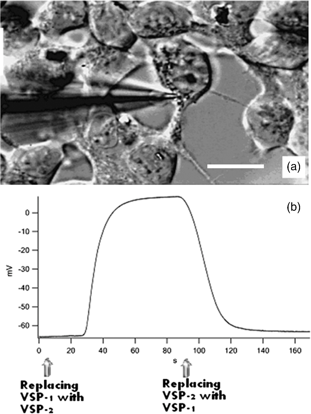

4. Summary

Detection and quantification of changes in PMP, in image and nonimage presentation at an individual based resolution is discussed without focusing on specific biological mechanisms. These changes, induced by high potassium solution, examined via the efficiency of FRET from coumarin (CC2-DMPE) and oxonol [DiSBAC2(3)], using both FI and FP measurements. Measurements were performed, before and after the induction of membrane depolarization on the same treated cells, while being arrested in their picowells. This approach ensured the attribution of the measured data individually to each investigated cell in suspension and hence enabled the examination of cell heterogeneity in regard to changes in PMP.

Cellular heterogeneity affects the performance of bioprocesses and plays an important role in organism-level outcomes. In many cases, cell–cell variability becomes evident through the ability of the cell to change its function over time. Current methodologies facilitate detection of changes in PMP in individual cells upon treatment, and correlation with other cellular functions such as cytoplasmic free ${Ca}^{(2 +)}$ and mitochondrial membrane potential, by multiparametric measurements.

Additionally, in the frame of the present work, i.e., cell models and fluorophores, it has been demonstrated that FP is indeed sensitive to changes in distance between membrane CC2-DMPE (coumarin) and DiSBAC2(3) (oxonol) dyes, and that FP based $E %$ -images might be more spatially contrastive than FI based $E %$ -images and hence complement the latter.

The fact that intracellular content is inhomogeneous, and thus highly scattering, seems to play in favor of FP based $E %$ measurement when the assessment of $E %$ in labeled cells is considered, particularly when inspected via wide field illumination. Minimizing artifacts due to photobleaching (which frequently occurs in fluorescence microscopy) might play in favor of the assessment of $E %$ via FP as well, since FP is generally indifferent to the number of fluorescing molecules, while FI is not.

Last but not least, the recruitment of FLIM for FRET measurement in HTS and drug discovery is still under intense debate. Some, unequivocally reject this possibility mainly because of the very long acquisition time needed, and equally, because of the complexity of system preparation and calibration, as well as interpretation of results. Those more optimistic believe that technological advances in excitation sources, detectors, data processing, and analysis, may increase the chances for FRET-FLIM to become more accessible.

On the other hand, the system described here is believed to be fairly accessible due to its simplicity, its being user friendly and its relatively low cost, whether whole cell or image analysis is used. In this regard, the possibility of assaying PMP heterogeneity in individual cells in suspension, as a complement (to other Vm imaging approaches) measure in HCS applications, is under examination at present.

Acknowledgments

This study was endowed by the Bequest of Moshe-Shimon and Judith Weisbrodt.

References

1.

F. M. Ashcroft, Ion Channels and Disease, Academic Press, San Diego, CA (2000). Google Scholar

2.

J. E. Gonzálezet al., “Cell-based assays and instrumentation for screening ion-channel targets,” Drug Discovery Today, 4 (9), 431 –439 (1999). http://dx.doi.org/10.1016/S1359-6446(99)01383-5 DDTOFS 1359-6446 Google Scholar

3.

N. FertigC. Farre, “Renaissance of ion channel research and drug discovery by patch clamp automation,” Future Med. Chem., 2 (5), 691 –695 (2010). http://dx.doi.org/10.4155/fmc.10.183 FMCUA7 1756-8919 Google Scholar

4.

D. C. CamerinoD. TricaricoJ.-F. Desaphy, “Ion channel pharmacology,” Neurotherapeutics, 4 (2), 184 –198 (2007). http://dx.doi.org/10.1016/j.nurt.2007.01.013 NEURNV 1878-7479 Google Scholar

5.

K. Sollyet al., “Miniaturization and HTS of a FRET-based membrane potential assay for K(ir) channel inhibitors,” Assay Drug Dev. Technol., 6 (2), 225 –234 (2008). http://dx.doi.org/10.1089/adt.2008.123 1540-658X Google Scholar

6.

G. C. Terstappenet al., “Screening technologies for ion channel drug discovery,” Future Med. Chem., 2 (5), 715 –7302010 http://dx.doi.org/10.4155/fmc.10.180 FMCUA7 1756-8919 Google Scholar

7.

E. NeherB. Sakmann, “Single channel currents from membrane of denervated frog muscle,” Nature, 260 799 (1976). http://dx.doi.org/10.1038/260799a0 NATUAS 0028-0836 Google Scholar

8.

J. Dunlopet al., “High-throughput electrophysiology: an emerging paradigm for ion-channel screening and physiology,” Nat. Rev. Drug Discovery, 7 (4), 358 –368 (2008). http://dx.doi.org/10.1038/nrd2552 NRDDAG 1474-1776 Google Scholar

9.

L. B. Cohen, “Changes in neuron structure during action potential propagation and synaptic transmission,” Physiol. Rev., 53 (2), 373 –418 (1973). PHREA7 0031-9333 Google Scholar

10.

Z. Krasznaiet al., “Flow cytometric determination of absolute membrane potential of cells,” J. Photochem. Photobiol. B, 28 (1), 93 –99 (1995). http://dx.doi.org/10.1016/1011-1344(94)07099-A JPPBEG 1011-1344 Google Scholar

11.

C. WolffB. FuksP. Chatelain, “Comparative study of membrane potential-sensitive fluorescent probes and their use in ion channel screening assays,” J. Biomol. Screen., 8 (5), 533 –543 (2003). http://dx.doi.org/10.1177/1087057103257806 JBISF3 1087-0571 Google Scholar

12.

K. Liuet al., “High-throughput screening for Kv1.3 channel blockers using an improved FLIPR-based membrane-potential assay,” J. Biomol. Screen., 15 (2), 185 –195 (2010). http://dx.doi.org/10.1177/1087057109356209 JBISF3 1087-0571 Google Scholar

13.

J. E. GonzálezR. Y. Tsien, “Voltage sensing by fluorescence resonance energy transfer in single cells,” Biophys. J., 69 (4), 1272 –1280 (1995). http://dx.doi.org/10.1016/S0006-3495(95)80029-9 BIOJAU 0006-3495 Google Scholar

14.

S. Damjanovichet al., Mobility and Proximity in Biological Membranes, 225 –326 CRC Press, Boca Raton, Florida (1994). Google Scholar

15.

M. Cohen-Kashiet al., “Fluorescence resonance energy transfer measurements on cell surface via fluorescence polarization,” Biophys. J., 83 (3), 1395 –1402 (2002). http://dx.doi.org/10.1016/S0006-3495(02)73910-6 BIOJAU 0006-3495 Google Scholar

16.

M. Cohen-KashiY. NamerM. Deutsch, “Fluorescence resonance energy transfer imaging via fluorescence polarization measurement,” J. Biomed. Opt., 11 (3), 034015 (2006). http://dx.doi.org/10.1117/1.2209955 JBOPFO 1083-3668 Google Scholar

17.

M. A. RizzoD. W. Piston, “High-contrast imaging of fluorescent protein FRET by fluorescence polarization microscopy,” Biophys. J., 88 (2), L14 –L16 (2005). http://dx.doi.org/10.1529/biophysj.104.055442 BIOJAU 0006-3495 Google Scholar

18.

J. A. Levittet al., “Fluorescence lifetime and polarization-resolved imaging in cell biology,” Curr. Opin. Biotechnol., 20 (1), 28 –36 (2009). http://dx.doi.org/10.1016/j.copbio.2009.01.004 CUOBE3 0958-1669 Google Scholar

19.

D. R. Matthewset al., “Time-lapse FRET microscopy using fluorescence anisotropy,” J. Microsc., 237 (1), 51 –62 (2010). http://dx.doi.org/10.1111/(ISSN)1365-2818 JMICAR 0022-2720 Google Scholar

20.

D. R. Matthewset al., “A multi-functional imaging approach to high-content protein interaction screening,” PLoS One, 7 (4), e33231 (2012). http://dx.doi.org/10.1371/journal.pone.0033231 1932-6203 Google Scholar

21.

A. N. Baderet al., “Homo-FRET imaging as a tool to quantify protein and lipid clustering,” Chemphyschem, 12 (3), 475 –483 (2011). http://dx.doi.org/10.1002/cphc.201000801 CPCHFT 1439-4235 Google Scholar

22.

M. Deutschet al., “A novel miniature cell retainer for correlative high-content analysis of individual untethered non-adherent cells,” Lab Chip, 6 (8), 995 –1000 (2006). http://dx.doi.org/10.1039/b603961h LCAHAM 1473-0197 Google Scholar

23.

J. E. GonzálezR. Y. Tsien, “Improved indicators of cell membrane potential that use fluorescence resonance energy transfer,” Chem. Biol., 4 (4), 269 –277 (1997). http://dx.doi.org/10.1016/S1074-5521(97)90070-3 CBOLE2 1074-5521 Google Scholar

24.

J. Pawley, Handbook of Biological Confocal Microscopy, –792 3rd ed.Springer, USA (2006). Google Scholar

25.

F. Perrin, “La fluorescence des solutions,” Ann. Phys. Paris, 12 169 –175 (1929). Google Scholar

26.

B. Valeur, Molecular Fluorescence: Principles and Applications, 2nd ed.Wiley-VCH Verlag GmbH, Weinheim, Germany (2001). Google Scholar

27.

The Biophysical Interdisciplinary Jerome Schottenstein Center for the Research and Technology of the Cellome, Demonstration of LCA functions ( (2013) http://www.jsc.ph.biu.ac.il/demonstration-of-lcafunctions/ Google Scholar

28.

M. Deutschet al., “Fluorescence polarization as a functional parameter in monitoring living cells: theory and practice,” J. Fluoresc., 12 25 –44 (2002). http://dx.doi.org/10.1023/A:1015355018449 JOFLEN 1053-0509 Google Scholar

29.

J. R. Lakowicz, Principles of Fluorescence Spectroscopy, 475 3rd ed.Springer, USA (2006). Google Scholar

Citation Download Citation

Tzachi Sabati, Bat-Sheva Galmidi, Alon Korngreen, Naomi Zurgil, and Mordechai Deutsch "Real-time monitoring of changes in plasma membrane potential via imaging of fluorescence resonance energy transfer at individual cell resolution in suspension," Journal of Biomedical Optics 18(12), 126010 (16 December 2013). https://doi.org/10.1117/1.JBO.18.12.126010

Published: 16 December 2013

Access the abstract

JOURNAL ARTICLE
11 PAGES

DOWNLOAD PAPER SAVE TO MY LIBRARY

GET CITATION

CITATIONS

Cited by 2 scholarly publications.

Explore citations on Lens.org

RIGHTS & PERMISSIONS

Get copyright permission Get copyright permission on Copyright Marketplace

KEYWORDS

Fluorescence resonance energy transfer

Plasma

Molecules

Polarization

Luminescence

Microscopes

Polarizers

1.

Introduction

1.1.

Mechanism and Theory

Eq. (1)

Eq. (2)

Eq. (3)

Eq. (4)

2.

Experimental

2.1.

Materials

2.2.

LiveCell™ Array (LCA)

Fig. 1

2.3.

Preparation of HEK-293 Cell Suspension

Fig. 2

2.4.

Cell Staining CC2-DMPE (Coumarin), DiSBAC2 (3) (Oxonol)

2.5.

Cell Loading and Solution Presentation into the LCA

2.6.

Optical Observations

2.6.1.

Measurement system

2.6.2.

Preparation of microscope for FP measurement

2.6.3.

Acquisition of images of FP from FP components

2.6.4.

Formation of FP and FI images

Eq. (5)

Eq. (6)

2.6.5.

Formation of E images

Eq. (7)

Eq. (8)

3.

Results and Discussion

3.1.

Pre- and postdepolarization FI and FP images

3.2.

Acquisition of Intensity Images from the FP Components

Fig. 3

3.3.

Analysis Based on FI and Polarization

Fig. 4

3.4.

E%-Images

Fig. 5

Fig. 6

3.5.

Direct Membrane Potential Measurements

Fig. 7

4.

Summary

Acknowledgments

References

Show All Keywords

Keywords/Phrases

Search In:

Publication Years

Cell Staining CC2-DMPE (Coumarin), DiSBAC₂ (3) (Oxonol)

$E %$ -Images