
|
|
1.IntroductionIn the past 10 years, clinical studies have shown that multispectral-based imaging technologies have outperformed the gold standard white light imaging method in terms of early cancer detection specificities and sensitivities.1–4 However, such multispectral methods have limited themselves by comparing the differences in the amplitudes of two to three emission wavelengths in the known ranges associated with certain fluorophores, such as nicotinamide adenine dinucleotide plus hydrogen (NADH) and flavin adenine dinucleotide (FAD), collagen, oxy- and deoxy-hemoglobin, etc.5–7 As a result, researchers have expanded the wavelength range to more than 100 spectral channels for each image pixel using a so-called hyperspectral technique.8–12 The hyperspectral image has been reported to be useful not only for aiding cancer detection for diagnostic purposes, but also for determining the tumor margin, evaluating the tumor base after tumor resection, and surveying and examining a vast area in a less invasive manner to provide a global screen for early cancer detection.9 Recently, we devised a microscope-based relay-lens hyperspectral imaging (HSI) system that has proven feasible for projecting the image plan from an optical system, such as a microscope, to an image acquisition unit [e.g., a charge-coupled device (CCD) camera]. The scanning of the image plan can be achieved using a relatively low-cost moving platform to move the relay-lens system with less precision because the scanned image plan has first been magnified through the projection optical path.13 However, the acquisition from hyperspectral images may reflect a complex mixture of different sources. For example, the mixture can come from the underlying reorganization of biochemical fluorophores in and around a tumorigenesis area.14 Such a reorganization includes an increased metabolism (as reflected by the increasing NADH) due to neoplastic development, a collapsed collagen matrix caused by tumor infiltration, and decreasing FAD concentration due to tissue remodeling. On the other hand, some excited fluorophores irrelevant to cancerization, as well as optical interferences caused by the imaging hardware, such as optical noise, reflection, scattering, and refraction, can also be included in the image mixture. As a result, it should be noted that the intensity alteration at a specific wavelength might result from the net effect of the mixture of different biochemical fluorophores and thus yield different results depending on how the HSI data are projected. A recent approach that uses independent component analysis (ICA) to process the biomedical signal and image data was successfully applied to electroencephalography (EEG) and functional magnetic resonance imaging (fMRI) data to separate the mixture of these data into independent brain blood oxygenation-level dependent (BOLD) activities, as well as the underlying electrical oscillations associated with specific brain processes.15–17 Here, we used ICA to decompose the HSI data obtained from 31 oral cancer tissue sections that contained well-developed and identifiable keratinized tissues from the fixed, excised oral cancer biopsies of 30 patients. We hypothesized that after separating the distinct spectral features associated with different molecules as well as the optical interferences, we would be able to easily identify the independent spectral component associated with the keratinized tissue given that ICA provides both the spatial and spectral information for each of the independent components, showing which area in the tissue contains what characteristic spectrum.15,17 After the independent spectral components of the keratinized tissues from the different patients/samples were identified, we could further test the consistency of the keratinized tissue-related spectra across different patients using a simple correlation analysis, plotting the mean and standard deviation of the multisample spectra and computing the coefficient of variation (COV) across different wavelengths. In the past, a similar approach using principal component analysis (PCA) was also documented for analyzing the HSI data of cancerous tissues.18 We therefore also compared the ICA results to the principal spectral components derived using the PCA method. The results show that the ICA method extracted more consistent keratinized tissue-related spectra with much higher correlations at both excitation wavelengths. 2.Microscope-Based Hyperspectral Imaging SystemA microscope-based HSI system (for more details, see Hsieh et al.13) was used to produce the HSI data of thin, frozen sections cut from excised oral cancer specimens. Briefly, a regular inverted fluorescence microscope was connected to a custom-designed and manufactured embedded relay-lens system capable of decomposing the two-dimensional (2-D) image of a thin-sliced object, one line at a time, into continuous spectra. By scanning through the entire 2-D object space, the relay-lens system produced a data cube with two dimensions in the spatial domain and one in the spectral domain (thus, x by y by ).8,13 The embedded relay-lens system consisted of a moving relay-lens set with a fixed slit of 30 μm width and a hyperspectrometer, spanning a spectral range of 400 to 1000 nm, to convert the slit image into continuous spectra. The slit image was relayed from the sliced object placed on the object platform of the microscope, which was lit by a Xenon light source filtered into two wavelength ranges, 330 to 385 nm and 470 to 490 nm, for excitation. Inside the embedded relay-lens system, a relay-lens was mounted on a stepping motor-controlled platform that could move the relay-lens in 10-μm steps to cover the entire field of view of the slice sample. On the other side of the embedded relay-lens system, an electron multiplying CCD (EMCCD) was mounted to take a snapshot of the HSI data projected from the image slit. The image resolution produced by the EMCCD was with 10-μm pixel size. As a result, the devised microscope-based HSI system generated a three-dimensional data cube with an in-plane resolution of in the spatial domain and 2.8 nm in the spectral domain. Finally, since a objective was used in the fluorescence microscope, this resulted in a spatial resolution of for this study. 3.Cancerous Tissue Preparations and LabelingThirty-one tissue sections of fixed oral cancer specimens, each containing clearly identifiable keratinized tissues, from 30 patients (aged , all males) were used to test the feasibility of finding the spectral fingerprints associated with keratinized tissues using ICA and PCA decomposition. These patients were all diagnosed with oral cancer with moderate- to well-differentiated squamous cell carcinoma in their oral cavity and/or tongue (stage II or higher). Before surgery, all patients were informed that the excised tissues would undergo hyperspectral image acquisition and be further processed by the ICA- and PCA-based image analysis procedure as a further examination. They also provided their signed informed consent. The use of the excised cancerous tissues as well as the image acquisition and analysis procedure for the HSI data were approved by the Institutional Review Board of China Medical University Hospital, Taichung Taiwan. All the procedures used complied with the Declaration of Helsinki. The regular pathological diagnosis procedure with hematoxylin and eosin (H&E) staining was used to prepare the section slices. An experienced pathologist (C.-I. J.) viewed the section slices under a regular microscope, rated the stage of cancer development, and labeled the regions with keratinization. The same sample slides then underwent hyperspectral image acquisition using the aforementioned system (see Sec. 2) and according to the locations labeled by the pathologist. The HSI data were then transferred to a computer server located in a different department for analysis by a different data analyst (J.-R. D.). Before the HSI data were transferred, the identification information linking the image data to the personal demographic data and the pathological diagnoses was removed for deidentification purposes. Note that the information regarding the spatial location of the keratinization in the samples was also not revealed to the data analyst while he was analyzing the data. 4.Data Preprocessing and Image ReconstructionBefore each section slide was scanned by the HSI system, two calibration images were obtained: (1) a dark field image with no light to the camera, which was used to remove the system noise and (2) a reference blank image, for which an area on the slide was scanned with all the layers of glass but without the tissue section sample. The latter calibration image was used to remove the nonuniformity caused by uneven illumination, periodic scan line stripping, and the reflection from the glass medium.11,13 After data preprocessing, the HSI data cube was first reconstructed into a series of 2-D image slices, each representing a 2-D autofluorescence intensity of the thin tissue slice at an emission wavelength. The two image dimensions corresponded to the spatial x- and y-axis of the 2-D object slice. In order to fit the limited memory space in the computer server used for the ICA decomposition, as well as to reduce the total computation time, each 2-D image slice was downsampled in space to one fourth () of the original image size (). Prior to downsampling, the 2-D image was spatially smoothed using a Gaussian spatial filter with a full width at half maximum of 2 pixels (1 μm) in each dimension. The processed data cube was then converted into a 2-D (, pixels by wavelengths) surrogate data set for further ICA decomposition. 5.ICA Decomposition and Component SelectionPrior to ICA decomposition, the surrogate data were first decomposed using PCA so as to determine the component number to be decomposed into via the ICA. The criterion to determine the component number was the principal dimension that preserved of the data variance. The PCA result was also stored so it could be compared to the ICA result. The surrogate data for each tissue sample were then decomposed using ICA into the previously determined component number. The Infomax ICA algorithm, as developed by Makeig et al.16 and implemented in the FMRLAB ( http://sccn.ucsd.edu/fmrlab),15 was used to decompose the surrogate data. The ICA process was used to maximize the independence by maximizing the sparseness or the kurtosis of each independent component (IC), which was derived via a linear decomposition using a 2-D inverse weight matrix. During the training phase of ICA decomposition, the optimization algorithms of gradient descent was used to iteratively adjust the elements of the inverse weight matrix so as to maximize the sparseness among the ICs. The iterative adjustment was halted when the total amount of adjustment was or when the maximum iteration had been reached ( was used here). Because of the data size, it could take up to 8 h for each ICA decomposition process to be completed. After the ICA process was finished, a linear back-projection was performed to multiply the input surrogate data with the inverse weight matrix to compute the independent spectral components that composed the HSI data. Each independent spectral component gave the spatial distribution in pixels, with relative intensities indicating the strengths (activations) with which the independent spectral component contributed to the data variance. This spatial distribution, also called the component map, was then standardized by removing the mean map and dividing it by the standard deviation of the component map. A threshold of a t-value was applied to find the highly significant pixels, and the characteristic autofluorescence spectrum across the entire wavelength span was computed by averaging the back-projected autofluorescence spectra of the selected highly participating pixels. As a result, the ICA gave two important pieces of information: one, in the spectral domain, showing the characteristic autofluorescence spectrum and the other, in the spatial domain, indicating which area in the tissues produced the derived independent spectrum. Given that the samples of cancerous tissue sections were prepared with H&E staining and annotated by an experienced pathologist, the spatial labels of keratinized tissues in the samples were finally compared with the results of the ICA components to determine the accuracy of the decomposition result. Since the ICA decomposition used all of the domain data in the process without any a priori knowledge regarding the spatial labels, the ICA-based spatial clustering process could thus be considered as blind. One IC that best matched the spatial locations of the labeled keratinized tissue in the oral cancer sample was selected as the target component. This same criterion was also used to select the principal spectral components from the PCA results. 6.Consistency of the Derived Autofluorescence Spectra of the Keratinized TissuesAfter the independent and principal components (PCs) with component maps overlapping with the keratinized tissues in the oral cancer samples were identified, the characteristic autofluorescence spectra associated with these selected components were computed for a further test of consistency. This consistency test was conducted by computing correlations between the characteristic spectra of any two of the 31 tissue samples (thus yielding 465 possible pairs). Finally, the mean correlations were computed for each of the four conditions [ (330 to 385 nm versus 470 to 490 nm)]. In addition, we also tested the consistency by plotting the standard deviations along with the mean spectrum obtained using different decomposition methods on the HSI data under different excitation wavelengths. These plots provided clear visualization of the consistency of the derived spectra by checking the envelope spanned by the standard deviations. In order to check in which part along the wavelength axis the derived spectra exhibited better consistency, we further computed the COV by computing the ratio of the standard deviation and mean spectrum at each wavelength. As a result, the COV could be plotted as a function of wavelength for each of the four conditions (). 7.ResultsThe data preprocessing and ICA decomposition were conducted on a Windows 2008 Server with an 8-core CPU and 24 GB of memory installed. A batch of routines implemented in the FMRLAB and running under a MATLAB® environment (Mathworks, MA) were used to derive the ICA results in a batch line mode. All the decomposition processes could be converged with training steps. For each HSI data cube, at least three decompositions were performed to guarantee the consistency of the outcomes. All the ICA results were stable, except for the fact that only the rankings of the output ICs might sometimes differ slightly in different decompositions. Generally speaking, ICA can be thought of as a grouping or clustering process that first separates the underlying independent processes (or sources) acquired in a mixed manner via an image or signal acquisition system and then groups the acquisition elements (e.g., pixels or voxels) to which a certain IC has significantly contributed. The example shown in this study is similar to the applications demonstrated by Duann et al.15 and Siegel et al.,19 wherein the spatial distributions of similar temporal behaviors were extracted from mixed data sets. Here the ICA process also provided two pieces of information, one being the autofluorescence spectrum that can be consistently found in the significant voxels and the other being the spatial distributions defining where those voxels are. In Fig. 1, the first column shows images of the same two tissue samples acquired with white light illumination. These images were identical to those on which the pathologist’s diagnoses were based. The white bar at the bottom of the image indicates the physical size of 100 μm. The second and third columns in Fig. 1 give the results of the ICA decomposition applied to the HSI data of two (out of the 31) tissue samples: sample #1 at the top and sample #2 at the bottom; excitation wavelength range #1 (330 to 385 nm) on the left and excitation wavelength range #2 (470 to 490 nm) on the right. The colored pixels in the spatial maps highlight the locations where their characteristic spectra highly resemble the spectrum shown at the bottom trace. The different colors (from red to yellow to white) indicate how strongly the individual pixels’ spectra resemble the bottom trace, with the white color indicating the highest and red indicating the lowest level of resemblance. Some of the independent spectral components revealing optical artifacts, such as background speckle noises, were also separated from the HSI data (Fig. 2). Note that these artifactual components also show specific fluorescence spectral patterns that might affect cancer tissue detection if not removed beforehand. On the other hand, the PCA also gives the spatial and spectral information, as did the ICA (the fourth and fifth columns in Fig. 1), but with different resultant characteristic autofluorescence spectra due to different decomposition principles. Fig. 1Independent component analysis (ICA) and principal component analysis (PCA) decomposition results of two exemplar cancerous tissue samples with the sample images acquired under two different excitation wavelength ranges (F1: 330 to 385 nm; F2: 470 to 490 nm). The first column gives the images of the two cancerous tissue samples acquired under white light illuminance; the second and third give the ICA results of the hyperspectral images (ICA at F1 and ICA at F2); and the fourth and fifth show the PCA results of the hyperspectral images (PCA at F1 and PCA at F2). The trace under each component image plot shows the autofluorescence spectrum of the keratinized tissues as highlighted in the images. The white bar at the bottom of the white light microscopic image indicates the size of 100 μm. 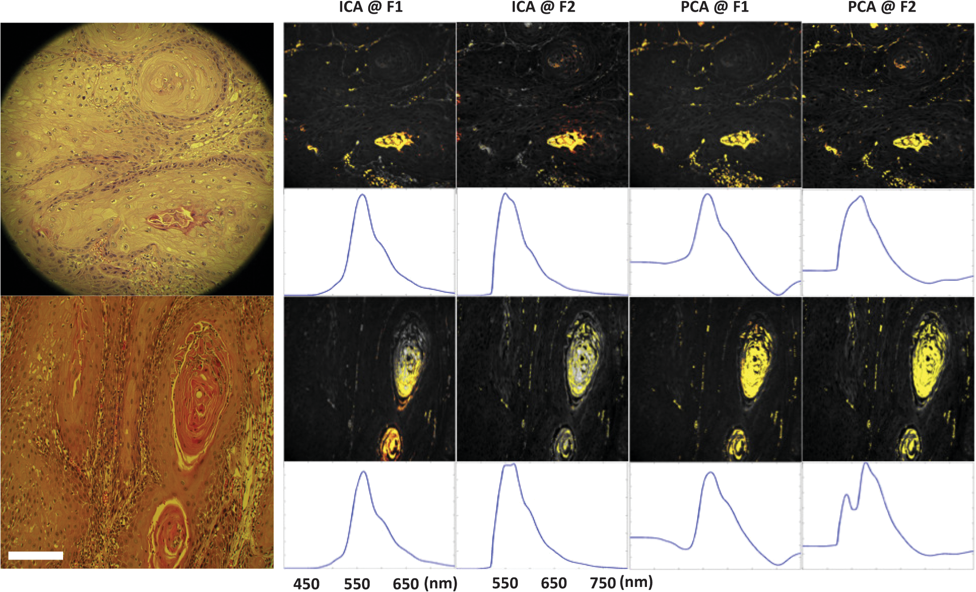 Fig. 2Example artifactual independent spectral components decomposed from the three-dimensional hyperspectral image data using ICA.  Figure 3 illustrates the mean spectra (thick black lines) and the standard deviation (shade) of the spectra associated with the keratinized tissues in the 31 tissue samples. As can be seen, ICA method results in more consistent characteristic spectra of keratinized tissues in both excitation wavelength ranges with smaller standard deviations across the entire wavelength range. ICA also gives sharper peaks in both cases. On the other hand, both ICA and PCA result in more consistent spectra from all HSI data under the excitation wavelength range of 470 to 490 nm. When applied to the HSI data excited by the wavelength range of 330 to 385 nm, both ICA and PCA result in higher uncertainty at the rising edges of the extracted characteristic spectra. Fig. 3Mean (solid lines) and standard deviation (shades) of the spectra of the keratinized tissues from the entire 31 oral cancer tissue samples as found using ICA and PCA decomposition methods. F1 indicates the excitation wavelength range from 330 to 385 nm and F2 indicates the excitation wavelength range from 470 to 490 nm.  In order to examine the consistency of each decomposition result across the entire spectrum, we further computed the COV by dividing the standard deviation of the resultant spectra with the mean spectra at each wavelength across different tissue samples. As a result, the COVs are plotted as a function of wavelength in Fig. 4. The COVs of ICA results are plotted in red and the COVs of PCA are plotted in blue; the solid lines depict the results decomposed from the HSI data excited by the wavelength range of 330 to 385 nm and the broken lines the results decomposed from the HSI data excited by the wavelength range of 470 to 490 nm. The results again show that the resulting spectra from ICA decomposition are quite consistent across different specimens (COVs for most of the wavelength range). However, the PCA decomposition gives only consistent spectra up to 650 nm and then the COVs increase largely and reach peaks at 700 nm for the HSI data excited with wavelength range of 330 to 385 nm and 760 nm for the HSI data excited with wavelength range of 470 to 490 nm. Fig. 4Coefficient of variation of the resulting spectra as a function of wavelengths of the two decomposition methods applied to the hyperspectral imaging data excited at different wavelength ranges. The red lines show the results of ICA decomposition and the blue the results of PCA decomposition. Solid lines indicate the results of the excitation wavelength range of 330 to 385 nm and broken lines the excitation wavelength range of 470 to 490 nm.  Table 1 gives the mean correlation coefficients between the characteristic autofluorescence spectra of any two of the sample tissues derived by different decomposition methods applied to the HSI data and at different excitation wavelength ranges. As can be seen, the ICA applied to the HSI data acquired at excitation wavelengths ranging from 470 to 490 nm yields the most consistent spectral fingerprints (with the highest mean correlation and lowest standard deviation) of keratinized tissues in the oral cancer tissue sections as compared to other conditions. On average, the ICA method outperformed the PCA method when applied to the HSI data acquired at both excitation wavelength ranges ( for both excitation wavelength ranges). Table 1Mean correlation coefficients (mean±standard deviation) between the autofluorescence spectra of the 10 sample tissues derived via various decomposition methods applied to different hyperspectral image data obtained at different excitation wavelength ranges.
8.Discussion and ConclusionAlthough autofluorescence spectroscopy has long been used to differentiate cancerous tissues from normal tissues, the reported evidence in the literature and the detection criteria used in commercially available testing devices are sometimes incompatible. As summarized by Ramanujam,20 distinct excitation wavelengths are needed in order to elicit maximal emission wavelengths for different endogenous fluorophores. As a result, any approach that targets different cancerization-related endogenous fluorophores may use different excitation wavelengths and find peak differences at different maximal emission wavelengths, thereby facilitating the ideal differentiation between cancerous and normal tissues. In order to have a more complete view using the characteristic autofluorescence spectroscopy associated with the endogenous fluorophores related to cancer development, it might be desirable to look at a wider spectrum so as to establish spectral biomarkers for cancer diagnosis and staging.11 In light of this, researchers are now actively pursuing imaging devices and data analysis strategies for HSI.8 However, one of the main obstacles in extracting reliable biomarkers for different biochemical fluorophores is the complex mixture of inputs during the acquisition of HSI data. The HSI data acquisition may involve autofluorescence emitted from various fluorophores, such as NADH, FAD, collagen matrix, elastin, etc., and other optical interferences. The autofluorescence of irrelevant fluorophores, as well as the artifacts, may sometimes contaminate the autofluorescence spectrum of the targeted fluorophores and, in turn, deteriorate the reproducibility of the resulting spectrum. Such a mixture problem would also affect traditional analysis methods in which the differences in fluorescence intensity at certain wavelengths that are excited at UV or other wavelengths are used to differentiate cancerous from normal tissue. On the other hand, the decrease or increase of fluorescence intensity is a measure relative to the baseline. As such, whether or not a reliable baseline can be obtained is critical to the validity of a traditional analysis method. Therefore, removing the effects of possible baseline drifting and separating the overlapping effects of two or more driving factors on the fluorescence intensity changes at the same emission wavelengths should shed light on the search for more reliable autofluorescence biomarkers for any fluorophores that actively participate in cancerization. To achieve this goal, one may consider using an algorithm, such as ICA or PCA, to separate and summarize the portions of data variance from a more specific process of cancerization. Such algorithms can separate the input data into components with minimum overlap in terms of statistical properties. For example, PCA, in general, finds a smaller set of uncorrelated variables that gives as good representation as possible based on second-order statistics.21 It thus tries to summarize as much data variance as possible into only the top few PCs. To achieve this, PCA finds this first PC that accounts for the largest possible variance, and each succeeding component in turn accounts the highest possible variance under the constraint that it be orthogonal to the preceding components. As a result, PCA can be efficiently implemented using, for example, singular value decomposition to convert a set of observations of possibly correlated variables into a set of linearly uncorrelated variables. ICA, on the other hand, separates the observation into statistically independent components based on higher-order statistics (e.g., kurtosis). To achieve this, ICA uses the algorithms to maximize the non-Gaussianity of the estimated components, which are not necessarily orthogonal to each other.22 Such nonorthogonal transforms that are sensitive to the higher-order statistics may help to fit into the detail structures of the data variance and find the underlying true sources.23 In the past, PCA has been used to separate underlying spectroscopic processes in fluorescence emission spectral data;18 the PCA method has been known to efficiently summarize data variance using the first few PCs (usually, the first five PCs tend to account for >90% of data variance). It may thus be likely that one PC can combine more than one characteristic autofluorescence spectrum in the HSI data. How many and which characteristic spectra would be combined in a PC depends on the variance of the different principal spectral components and could vary across different HSI data. Consequently, as shown in this study, the PCA resulted in less consistent spectral fingerprints, even though the keratinized tissues in the tissue sections could be identified equally well from the HSI data. Compared to PCA, ICA has proved capable of decomposing electroencephalograph/megnetoencephalograph (EEG/MEG) and fMRI data into reliable ICs that demonstrate more consistent behavior across different subjects.15–17 The extracted ICs represented more purified brain EEG electrical oscillations and fMRI BOLD signals with less contamination from other irrelevant brain activations and/or artifactual components. In line with these findings, our ICA results revealed more consistent independent characteristic spectra associated with keratinized tissues in the HSI data from various cancer specimens of different patients. Although the present study has proven the process of ICA useful for reliably separating the independent characteristic spectra associated with keratinized tissues from the mixture of HSI data of different oral cancer tissue sections, this can only be considered a first step toward finding the hyperspectral fingerprints for cancer development and diagnosis. As keratinized tissues are mostly found during very late stages of cancerization and the biochemical composition seems to be more consistent in keratinized tissues,24,25 the ability to detect the presence of keratinized tissues is of no direct diagnostic value for early cancer detection. Keratinized tissues were used in this study simply to test the feasibility of the proposed method with easily identifiable ground truth. To apply the proposed approach to the HSI data of other types or stages of cancerous tissue, samples should be straightforward. Basically, the same procedure still applies. Therefore, an important next step would be to test if any hyperspectral fingerprints can be found for different molecules that can reflect the stages of cancer development. It would be valuable, moreover, to devise a portable system that could be used in physicians’ offices to help clinicians screen suspicious spots of epithelial mucosa in, for example, the oral cavity and thereby determine whether or not a biopsy is necessary. AcknowledgmentsThe authors would like to thank Mr. Yao-Fang Hsieh and Mr. Chih-Hsien Chen for their constant calibrations of the hyperspectral imaging device. This study was supported in part by the National Science Council (NSC 100-2218-E-039-001) of Taiwan. J.R.D., M.O.-Y., Y.-J. L., and J.-C.C. were further supported by the “Aim for the Top University Plan” of National Chiao Tung University and the Ministry of Education of Taiwan. ReferencesP. M. Laneet al.,
“Simple device for the direct visualization of oral-cavity tissue fluorescence,”
J. Biomed. Opt., 11
(2), 024006
(2006). http://dx.doi.org/10.1117/1.2193157 JBOPFO 1083-3668 Google Scholar
P. Sharmaet al.,
“The utility of a novel narrow band imaging endoscopy system in patients with Barrett’s esophagus,”
Gastrointest. Endosc., 64
(2), 167
–175
(2006). http://dx.doi.org/10.1016/j.gie.2005.10.044 GAENBQ 0016-5107 Google Scholar
M. A. Karaet al.,
“Endoscopic video-autofluorescence imaging followed by narrow band imaging for detecting early neoplasia in Barrett’s esophagus,”
Gastrointest. Endosc., 64
(6), 679
–685
(2005). http://dx.doi.org/10.1016/j.gie.2005.11.050 GAENBQ 0016-5107 Google Scholar
W. L. Curverset al.,
“Endoscopic tri-modal imaging for detection of early neoplasia in Barrett’s esophagus: a multi-centre feasibility study using high resolution endoscopy, autofluorescence imaging and narrow band imaging,”
Gut, 57
(2), 167
–172
(2008). http://dx.doi.org/10.1136/gut.2007.134213 GUTTAK 0017-5749 Google Scholar
R. Drezeket al.,
“Autofluorescence microscopy of fresh cervical-tissue sections reveals alternation in tissue biochemistry with dysplasia,”
Photochem. Photobiol., 73
(6), 636
–641
(2001). http://dx.doi.org/10.1562/0031-8655(2001)0730636AMOFCT2.0.CO2 PHCBAP 0031-8655 Google Scholar
Y. WuW. ZhengJ. Y. Qu,
“Time-resolved confocal fluorescence spectroscopy reveals the structure and metabolic state of epithelial tissue,”
Proc. SPIE, 6430 643013
(2007). http://dx.doi.org/10.1117/12.702450 PSISDG 0277-786X Google Scholar
G. Zonioset al.,
“Diffuse reflectance spectroscopy of human adenomatous colon polyps in vivo,”
Appl. Opt., 38
(31), 6628
–6637
(1999). http://dx.doi.org/10.1364/AO.38.006628 APOPAI 0003-6935 Google Scholar
R. A. Schultzet al.,
“Hyperspectral imaging: a novel approach for microscopic analysis,”
Cytometry, 43
(4), 239
–247
(2001). http://dx.doi.org/10.1002/(ISSN)1097-0320 CYTODQ 0196-4763 Google Scholar
H. Akbariet al.,
“Cancer detection using infrared hyperspectral imaging,”
Cancer Sci., 102
(4), 852
–857
(2011). http://dx.doi.org/10.1111/cas.2011.102.issue-4 CSACCM 1349-7006 Google Scholar
G. M. Palmeret al.,
“Optical imaging of tumor hypoxia dynamics,”
J. Biomed. Opt., 15
(6), 066021
(2010). http://dx.doi.org/10.1117/1.3523363 JBOPFO 1083-3668 Google Scholar
A. M. Siddiqiet al.,
“Use of hyperspectral imaging to distinguish normal, precancerous, and cancerous cells,”
Cancer, 114
(1), 13
–21
(2008). http://dx.doi.org/10.1002/cncr.23286 60IXAH 0008-543X Google Scholar
R. T. Kesteret al.,
“Real-time snapshot hyperspectral imaging endoscopy,”
J. Biomed. Opt., 16
(5), 056005
(2011). http://dx.doi.org/10.1117/1.3574756 JBOPFO 1083-3668 Google Scholar
Y. F. HsiehM. Ou-YangC. C. Lee,
“Finite conjugate embedded relay lens hyperspectral imaging system (ERL-HIS),”
Appl. Opt., 50
(33), 6198
–6205
(2011). http://dx.doi.org/10.1364/AO.50.006198 APOPAI 0003-6935 Google Scholar
C. F. Pohet al.,
“Fluorescence visualization detection of field alterations in tumor margins of oral cancer patients,”
Clin. Cancer Res., 12
(22), 6716
–6722
(2006). http://dx.doi.org/10.1158/1078-0432.CCR-06-1317 CCREF4 1078-0432 Google Scholar
J. R. Duannet al.,
“Single-trial variability in event-related BOLD signals,”
Neuroimage, 15
(4), 823
–835
(2002). http://dx.doi.org/10.1006/nimg.2001.1049 NEIMEF 1053-8119 Google Scholar
S. Makeiget al.,
“Mining event-related brain dynamics,”
Trends Cogn. Sci., 8
(5), 204
–210
(2004). http://dx.doi.org/10.1016/j.tics.2004.03.008 TCSCFK 1364-6613 Google Scholar
M. J. McKeownet al.,
“Spatial independent activity patterns in functional MRI data during the Stroop color-naming task,”
Proc. Natl. Acad. Sci. U. S.A., 95
(3), 803
–810
(1998). http://dx.doi.org/10.1073/pnas.95.3.803 1091-6490 Google Scholar
N. Ramanujamet al.,
“Cervical pre-cancer detection using a multivariate statistical algorithm based on laser induced fluorescence spectra at multiple excitation wavelengths,”
Photochem. Photobiol., 64
(4), 720
–735
(1996). http://dx.doi.org/10.1111/php.1996.64.issue-4 PHCBAP 0031-8655 Google Scholar
R. M. Siegelet al.,
“Spatiotemporal dynamics of the functional architecture for gain fields in inferior parietal lobule of behaving monkey,”
Cereb. Cortex, 17
(2), 378
–390
(2007). http://dx.doi.org/10.1093/cercor/bhj155 53OPAV 1047-3211 Google Scholar
N. Ramanujam,
“Fluorescence spectroscopy of neoplastic and non-neoplastic tissues,”
Neoplasia, 2
(1–2), 89
–117
(2000). http://dx.doi.org/10.1038/sj.neo.7900077 1522-8002 Google Scholar
C. BugliP. Lambert,
“Comparison between principal component analysis and independent component analysis in electroencephalograms modelling,”
Biom. J., 48
(2), 1
–16
(2007). http://dx.doi.org/10.1002/bimj.200510285 BIJODN 0323-3847 Google Scholar
P. Comon,
“Independent component analysis, a new concept?,”
Signal Process., 36
(3), 287
–314
(1994). http://dx.doi.org/10.1016/0165-1684(94)90029-9 SPRODR 0165-1684 Google Scholar
T. P. Junget al.,
“Imaging brain dynamics using independent component analysis,”
Proc. IEEE, 89
(7), 1107
–1122
(2001). http://dx.doi.org/10.1109/5.939827 IEEPAD 0018-9219 Google Scholar
S. Kurokiet al.,
“Epithelialization in oral mucous wound healing in terms of energy metabolism,”
Kobe J. Med. Sci., 55
(2), E5
–E15
(2009). KJMDA6 0023-2513 Google Scholar
S. D. Silvaet al.,
“Fatty acid synthase expression in squamous cell carcinoma of the tongue: clinicopathological findings,”
Oral Dis., 14
(4), 376
–382
(2008). http://dx.doi.org/10.1111/j.1601-0825.2007.01395.x 1354-523X Google Scholar
|


