1.

Introduction

Optical coherence elastography (OCE) provides deformation or the material property mapping of soft tissue.^1,2 The addition of elastographic contrast may improve the inherent ability of optical coherence tomography (OCT) to differentiate the composition and structure of soft tissue.³ Moreover, the mechanical information extracted from OCE is important for analysis and identification of pathological changes in soft tissue. For example, OCE may provide high-resolution characterization of strains in arterial walls, which would be important complementary information for determining the stability of atherosclerotic lesions.⁴ There are two main categories of OCE techniques, phase-based methods^5,6 and speckle tracking techniques,^7–9 which rely on the structure of the speckle pattern when it is fixed. In general, speckle-tracking based OCE can measure greater deformation than phase-based OCE methods as phase-based OCE is limited by the phase stability of OCT system¹⁰ and the phase wrapping induced by large physical deformations or high detected particle velocities within the imaging volume. Although phase unwrapping could extend the measurement range of the phase-based method, it is difficult to apply due to noise corruption or discontinuity of the wrapped phase maps in OCT imaging.^6,11 The principle of speckle tracking techniques has been previously described by Schmitt.¹ Briefly, the speckle can be temporally tracked by quantifying the displacement via cross correlation of the OCT images of prestressed and stressed tissue samples. However, the resolution for the displacement calculation was limited to 1 pixel and no strain elastograms were given, as the process of strain calculation by differentiating the displacements was very sensitive to noise. Kirkpatrick et al.¹² demonstrated that a maximum likelihood speckle shift estimator is superior than cross correlation, when the tissue motion between frames is less than 0.8 pixels. However, in practice, it is difficult to estimate the pixel shift a priori. Moreover, if the deformation values have a wide range from subpixels to pixels, the maximum likelihood will not be effective. Another drawback of the existing speckle tracking methods is the use of numerical differentiation of displacements to obtain strains. This procedure is noise sensitive as any error in the displacement measurement will be amplified in its strain calculation.¹³ Due to these complications, the large majority of the present speckle-tracking based OCE techniques has not been verified for their measurement accuracy. Therefore, more advanced algorithms are required to improve the measurement resolution and accuracy. We aim to develop a robust speckle-tracking based OCE methodology with subpixel resolution and improved strain measurement accuracy.

Digital image correlation (DIC)^14–16 is widely accepted for mechanical testing. The basic principle of DIC includes the tracking of the same points (or pixels) between the two images recorded before and after deformation. When DIC is applied to continuum mechanics, strains can be simultaneously obtained with displacements.¹⁷ Simultaneous computation of displacement and strain differentiates DIC from regular speckle tracking algorithms employed in image processing when compared to pattern recognition algorithms. DIC has been used to measure the material properties of biological tissues and biomaterials.¹⁸ This was accomplished by employing artificial speckle patterns on the surface of the specimen. DIC can be implemented if the speckle pattern deforms together with the specimen surface as a carrier of deformation. Under the condition of small perturbations due to time or mechanical loading where the changes of the speckle pattern between frames are small and free of discontinuities, we hypothesize that the DIC algorithm can be applied to OCT images, resulting in optical coherence elastograms. Such a hypothesis can be tested via static loading using low-frame rating imaging systems and when in practice, it will require high-frame rate devices to address dynamic loading conditions. Furthermore, DIC requires high-spatial-frequency information of the speckle to optimize the cross-correlation calculation. Therefore, image contrast and nonuniform distribution of speckle may affect the resolution and accuracy of the results.^19,20 The contrast and brightness of OCT images decrease with imaging depth, which may also result in a decreasing correlation coefficient as a function of depth. The prerequisite for the effectiveness of this DIC-based OCE is that the speckle patterns are correlated. The correlation stability of the OCT speckle images free of load is evaluated. The focus of this article is to present this novel DIC-based OCE technique for deformation imaging of soft tissue. The technique was evaluated in terms of system error and differentiation of various biological composite materials. Advantages, limitations, and further development are also discussed.

2.

Materials and Methods

2.2.

OCE Procedure and System Calibration

The OCE system consists of a custom polygon-based swept-source OCT (SSOCT) system and a loading structure. A diagram of the OCT system is shown in Fig. 1(a). The OCT system has a 36-kHz A-scan frequency, $\sim 15\text{-}\mu \text{m}$ axial resolution in air, and $\sim 25\text{-}\mu \text{m}$ lateral resolution determined by the focal spot size of the imaging lens (LSM03, Thorlabs, Newton, New Jersey). A photo of the loading structure under the scanning lens is shown in Fig. 1(b).

Fig. 1

(a) Schematic diagram of the swept-source optical coherence tomography (SSOCT) system. (b) Photo of the loading structure. Symbols on (a): BD, balanced photodetector; C, collimator; CIR, circulator; D, photodetector; FBG, fiber bragg grating; GVS, galvoscanner; L1 and L2, lenses; PC, polarization controller; SOA, semiconductor optical amplifier. The list of parts in (b): (1) OCT galvoscanner with an imaging lens. (2) Optical window. A tissue sample is underneath it. (3) Compression plate. (4) Translation stage. Compression load is applied by translating the compression plate downwards.

The loading structure shown in Fig. 1(b) is made of a plate fixed to a linear translation stage. A 20-mm-diameter hole was fabricated on the plate, and a 1.2-mm-thick cover slip was glued to the bottom of the plate to allow the transmission of light and application of the load. Static load was applied by adjusting the translation stage downwards. DIC calculations were performed on two consecutive frames of OCT images of a sample before and after deformation. A schematic diagram of OCE procedure is shown in Fig. 2. The sample was cut into $\sim 5\times 5{\mathrm{mm}}^2$ pieces and covered with solution to match the refractive index if necessary. Preload was applied while the first OCT image was taken.⁸ Preloading was applied to ensure that the glass window was in contact with tissue and decrease the correlation noise.²³ It was applied by moving the compression plate down a certain distance, usually in the range of a few microns depending on the shape of the sample, beyond the point of first contact. The two frames of OCT images taken under preload and compressive load were then computed by DIC to obtain displacement distribution maps and elastograms of normal strains and shear strain simultaneously.

Fig. 2

Diagram of the optical coherence elastography (OCE) procedure.

We first evaluated the system error by processing two consecutive images of a phantom without applying a load. The phantom was $\sim 10\text{-}\mathrm{mm}$ thick and made of RTV silicone (ELASTOSIL RT 601 A/B, WACKER, Germany) with ${\mathrm{TiO}}_2$ as an optical scatter. The concentration of ${\mathrm{TiO}}_2$ was $25\mathrm{mg}/\mathrm{ml}$, and the mixing ratio of A/B was 15:1, resulting in elastic modulus of $\sim 3060\mathrm{KPa}$.²⁴ The two frames of OCT image of the phantom were taken at an interval of $~1\mathrm{s}$. One of the images is displayed in Fig. 3(a). The displacements and strains in this sample were expected to zero as no load was applied. Therefore, the resultant OCE images indicate the inherent measurement error of the system. Figure 3(b) demonstrates the correlation coefficient in a region of interest (ROI). Correlation coefficients $>0.92$ were observed throughout the ROI indicating a high correlation in the speckle pattern. The displacement in the axial and lateral direction is shown in Figs. 3(c) and 3(d), respectively, from which it can be seen that the system error for displacement measurement was $<0.1$ pixels in axial direction and $<0.2$ pixels in lateral direction. The measurement error is slightly greater in the lateral direction, possibly due to jitter in the Galvo scanning mirror, subject to feedback mechanisms in its control loop. The normal strains in the axial direction and lateral direction are shown in Figs. 3(e) and 3(f), which demonstrate a measurement error of $<0.5\%$. We also evaluated the correlation changes of the speckle patterns with time. The phantom free of load was imaged with various time intervals of 0 to 15 min. The average and standard deviation of the correlation coefficients within the ROI was plotted with time in Fig. 3(g). The error bars demonstrated that the variations of the coefficient within the ROI are not significant. Although the correlation coefficient varies with time in general, it seems to be of a random nature. This random change could be explained by the random characteristics of speckles. The speckle pattern is sensitive to the system unstableness, such as minor vibrations in the optical table or jitter in the Galvo scanning mirror. The lowest correlation coefficient was 0.75 within the 15-min timeframe. A $C>0.6$ was defined as strong correlation as per previous publication.²⁵ Thus, results obtained when $C<0.6$ were considered to be poor data as decorrelation between the speckle patterns existed.

Fig. 3

OCE system evaluation by comparing two frames of optical coherence tomography (OCT) images taken at $\sim 1\text{-}\mathrm{s}$ time interval. (a) One of the OCT frames (nearly identical to the second frame); (b) correlation coefficient distribution between the two frames within a region of interest (ROI); (c) displacement in the axial direction; (d) displacement in the lateral direction; (e) normal strain in the axial direction; (f) normal strain in the lateral direction; (g) plot of the average and standard deviation of correlation coefficients within the ROI with time; (h) plot of the root mean square (RMS) contrast of the OCT image with depth; (i) plot of the correlation coefficient with depth. Scale bars on (a)–(f) 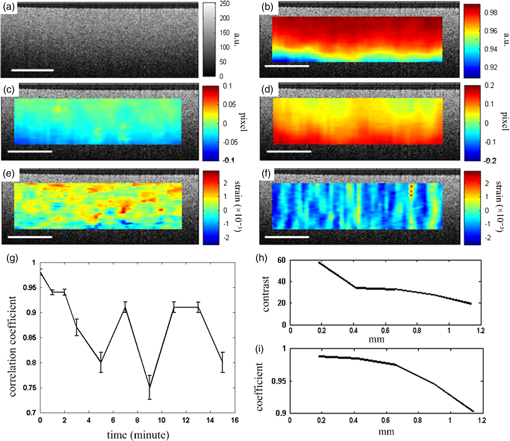$=1\mathrm{mm}$.

Due to light absorption of tissue, the intensity of the image decreases with depth. In this experiment, the total imaged depth was $\sim 1.2\mathrm{mm}$ representing 300 pixels in the axial direction. The changes of the root mean square (RMS) contrast²⁶ and correlation coefficient with depth were evaluated and plotted in Figs. 3(h) and 3(i). As estimated, the correlation becomes weaker with the decreasing of image contrast.

To calibrate the relationship between physical deformation and pixel shift in the OCE image domain, a homogeneous phantom made of candle gel and ${\mathrm{TiO}}_2$, with a thickness of $\sim 10\mathrm{mm}$, was tested. The resultant relationship was termed as the $\mu \text{m}/\text{pixel}$ ratio. A series of compressions ranging from 1 to 150 μm was applied to deform the phantom. The compressions were applied by adjusting the translation stage. The measurement results are shown in Fig. 4. One OCT image is shown in Fig. 4(a). The axial displacements of the sample undergoing 10-μm compression are overlaid on a structural image and shown in Fig. 4(b). The width of the ROI was $\sim 0.6\mathrm{mm}$, assuming that the refractive index of the sample was 1.4. The ROI includes 800 and 240 pixels in the horizontal and vertical directions, respectively. The 300 pixels evenly distributed within the ROI with 8-pixel interval were calculated by Eq. (1). The values of the pixels that are not directly calculated were obtained by interpolation. The displacement inflicted via the translation stage was 10 μm on the top surface of the phantom, which gradually decreased with depth. The measurement results in Fig. 4(b) do not show a gradual decreasing pattern in the axial direction as the variations of the displacement in the ROI were too small to be resolved by the DIC-based OCE algorithm. Figure 4(c) shows that the pixel shift in images linearly increases with the increasing of the compression. The horizontal coordinate of the “$x$” is the average displacement applied in the ROI, and the vertical coordinate is the average value in the ROI measured by OCE. For example, at 150-μm compression, the displacement distribution of the phantom is from 150 μm on the top surface linearly dropping to 0 at the bottom of the phantom. Thus, the average value within the ROI can be calculated by

$$[\text{displacement on top surface}]+(\text{displacement at the bottom of the}\mathrm{ROI})/2=[150\mu \text{m}+(150\mu \text{m}-\frac{150\mu \text{m}}{10\mathrm{mm}}·0.6\mathrm{mm}\left)\right]/2=145.5\mu \text{m}$$

neglecting the thickness above the ROI. There was $~9\mu \text{m}$ displacement variation within the ROI under 150-μm compression. Taking the average value in the curve fitting in Fig. 4(c) for the calibration will improve the calibration accuracy. The $\mu \text{m}/\text{pixel}$ ratio was calculated to be 5.8 based on the linear curve fitting. More specifically, one pixel shift between the two OCT images was caused by 5.8 μm deformation of the sample. The correlation coefficient decreases with the increasing of the displacement as shown in Fig. 4(d). The correlation coefficient was about 0.6 at 150 μm, which was considered to be the maximum measurable displacement. Maps of displacement in lateral and axial directions of the phantom under 150-μm compression are shown in Figs. 4(e) and 4(f). In the lateral direction, the scanned length was 5 mm including 1024 pixels and resulted in $4.9\mu \text{m}/\text{pixel}$. Negative values demonstrate that the ROI is on the left side of the center of the phantom. The axial displacements in Fig. 4(f) show a decreasing trend with depth as expected.

Fig. 4

System calibration. (a) An OCT image of a phantom. (b) Map of displacement in axial direction of the phantom under 10-μm compression. (c) Plot of measured pixel shift in images versus given displacement where $x$ indicates pixel shift obtained by digital image correlation (DIC)-based OCE at each given compression and straight line is the linear fitting of the data. This plot shows that 5.8-μm displacement induces 1 pixel change on OCT images. (d) Plot of correlation coefficient versus displacement. (e) Map of displacement in the lateral direction of the phantom under 150-μm compression applied from the top. Negative values demonstrate that the ROI is on the left side of the center of the phantom. (f) Map of the displacement in the axial direction of the phantom under 150-μm compression, demonstrating the gradual decrease of deformation from top of the ROI to the bottom. Scale bars 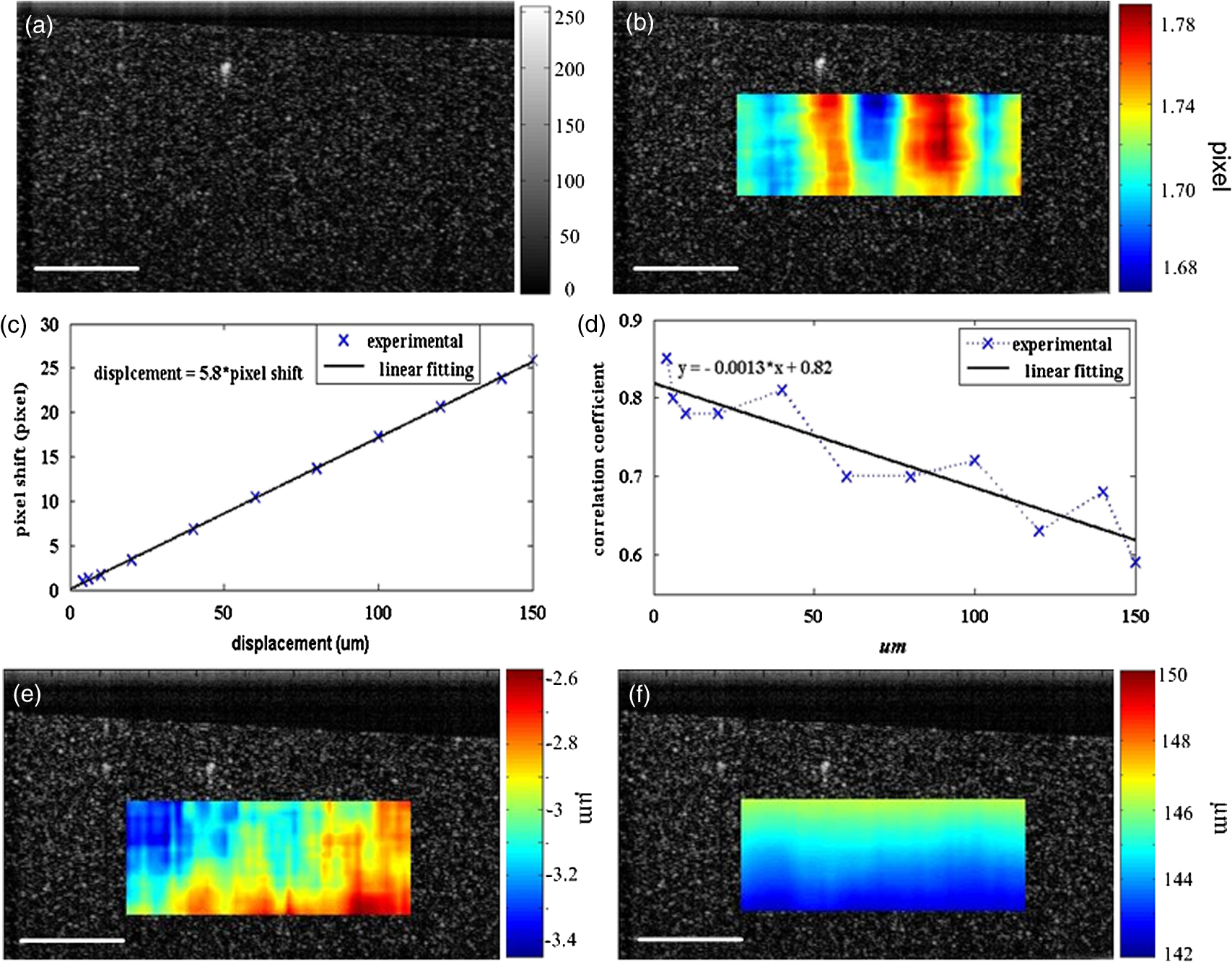$=1\mathrm{mm}$.

2.3.

Evaluation of OCE for Material Differentiation

A candle gel and ${\mathrm{TiO}}_2$ phantom including a small stiff part made of silicon and ${\mathrm{TiO}}_2$ were tested by the DIC-based OCE technique. To estimate the elastic modulus of the candle gel and the silicon inclusion, compression tests were conducted. Samples of $\sim 25{\mathrm{mm}}^2\times 3\mathrm{mm}$ thick were resected from the candle gel and silicon material, respectively. A load cell (FSH01045, FUTEK, Irvine, California) was fixed at the bottom of the loading structure as shown in Fig. 1(b). The 100-μm compression was applied to each sample by the translation stage while the load was recorded by the load cell. Then, the elastic modulus was estimated by $E=\frac{\sigma }{\epsilon }$ assuming linear elastic material, where $E$ is the Young’s modulus, $\sigma$ is the stress, and $\epsilon$ is the strain in the equation. The Young’s modulus ($E$) was experimentally derived to be 8.98 MPa for the small silicon inclusion and 2.99 MPa for the surrounding candle gel material. To make the candle gel phantom with stiff silicon inclusion, a few random sized pieces of the silicon phantom were cut off and embedded to the candle gel before it solidified. A photo of the phantom is shown in Fig. 5(a). A small piece enclosed by a rectangle on Fig. 5(a) was cut off for OCE experiment. The stiffer piece is vaguely visible in the OCT images of Figs. 5(b) and 5(c), which are taken before and after compression. The phantom was compressed by $~20\mu \text{m}$. Displacements and strains in the axial direction of an ROI obtained by the DIC-based OCE are shown in Figs. 5(d) and 5(e). It can be seen that the stiff block deforms less than the surrounding region. From the strain elastogram displayed in Fig. 5(e), the boundary of the stiff block is clearly visible. The strains generated on the block are significantly smaller than the strain on the surrounding material. A strain distribution map obtained by numerical derivation of the displacement is shown in Fig. 5(f), which is severely corrupted by noise. As it is difficult to estimate the strain distribution of the phantom which has such a nonregular shape inclusion, we conducted a finite element simulation using COMSOL4.3 to verify the OCE results. Isotropic linear elastic models were used in the simulation. Poisson’s ratio for both materials is 0.499 and Young’s modulus is 8.98 and 2.99 MPa, respectively, as per the experimental measurements. Under 20-μm compression, the normal strain distribution in the axial direction was displayed in Fig. 5(g). The pattern of the strain distribution matches well with the experimental results in Fig. 5(e). A large strain region above the inclusion is shown in green–blue in Fig. 5(e) and blue in Fig. 5(g). Discrepancy of the values between Figs. 5(g) and 5(e) is due to a few factors including: (1) shape: the geometry of the phantom in the simulation is not identical to the actual phantom, because the actual phantom, especially the stiff inclusion, does not have perfectly straight edges; (2) material of the phantom may not be homogeneous, as suggested by Fig. 5(d); (3) two-dimensional simulation was conducted while the actual phantom is a three-dimensional object; and (4) the material properties used in the simulation may differ from the actual values.

Fig. 5

OCE imaging of a phantom that has a stiff inclusion. (a) A photo of the phantom with stiff inclusions. The part in red rectangle was cut off for OCE test. (b) and (c) Two frames of OCT images of the phantom before and after compression. (d) Displacement in the axial direction overlaid on a structural image. (e) Axial strain elastogram overlaid on a structural image where the strain values on the stiffer block are between 0 and $-0.5\%$, which is smaller than the strains on the material surrounding it. The boundary of the stiff block is clearly visible. (f) Axial strain distribution obtained by numerical derivation of the displacement measured in (d). (g) Simulation of strain in the axial direction. The dashed line rectangular indicates the ROI in the OCE measurement. Scale bars on (b)–(g) $=1\mathrm{mm}$.

3.

Biological Tissue Imaging

The DIC-based OCE technique was applied to image biological tissues. Unlike the phantoms, where the fundamental shape could be reasonably controlled, the biological tissue did not have regular shapes. Thus, the load applied may not be uniformly distributed, resulting in complicated stress analysis. Therefore, only the strain distributions of these samples through the DIC-based OCE were investigated without detailed conformational analysis of stress distributions.

A chicken breast sample was imaged by the DIC-based OCE algorithm. A small piece containing a layer of fat on the top, a soft membrane in the middle, and a muscle layer at the bottom was imaged. The sample was compressed by 10 μm. Imaging results are shown in Fig. 6. Figure 6(a) is an OCT image of the sample. The three layers are labeled as F for fat, Me for membrane, and Mu for muscle, based on estimation, as clear boundaries are not visible on the OCT image. Due to the nonregular shape of the sample, the cover slip was only in contact with the right part of the top surface. Figure 6(b) shows the map of displacement in the axial direction. The displacement distribution varies from 9 to 10 μm. Figure 6(c) is the elastogram of normal strain in axial direction, which shows that the softer membrane has higher strain of $\sim 1\%$ comparing with almost zero strain on the top and bottom layers.

Fig. 6

OCE imaging of a chicken breast sample. (a) OCT image of the sample. F: fat layer, Me: membrane, Mu: muscle. (b) Displacement distribution in the axial direction. (c) Elastogram of normal strain in the axial direction, which shows the softer membrane in the middle. $\text{Scale bars}=1\mathrm{mm}$.

A cerebral aneurysm is a blood-filled dilation (balloon-like bulge) in the wall of the cerebral artery. Rupture of the cerebral aneurysm can cause hemorrhage to the brain with potentially fatal consequences. It is essential to understand the mechanical conditions and consequent stress distribution in arterial walls that involved in aneurysmal rupture. Local variations in the anisotropy and inhomogeneity of arterial tissues have not been examined in detail due to limitations of imaging and experimental approaches. Walraevens et al.²⁷ suggest that a compression test could be able to discriminate healthy from calcified aortic vascular wall tissue. In this work, a cerebral aneurysm sample using the DIC-based OCE was imaged as a feasibility study. The aneurysm sample was obtained under discarded human tissue exemption and had been fixed in formalin for several months before the OCE test. A photo of an aneurysm is shown in Fig. 7(a). The upper right corner of the sample was resected for the OCE test, which is shown in Fig. 7(b). The aiming beam indicates the imaged cross-section. One OCT image of the cross-section of the sample is shown in Fig. 7(c). Figure 7(d) is the histology of the cross-section correlating to Fig. 7(c). A dashed rectangular region is zoomed in Fig. 7(f). Figure 7(e) is the elastogram of normal strain in the axial direction overlaid on the OCT image. The ROI indicated by white arrows in Fig. 7(e) is correlated to the region indicated by black arrows in Fig. 7(d) where the adventitia and media have different structures. OCE image clearly shows the boundary of the adventitia layer, which is not clearly identified in OCT structural image in Fig. 7(c). The region indicated by a red asterisk is not processed because the speckle patterns are decorrelated. The sample was also imaged from the bottom side of Fig. 7(d). The elastogram of axial normal strains overlaid on an OCT image is shown in Fig. 7(g). A high strain region in blue indicated by a black arrow correlates to the local heterogeneity in the fibrotic aneurismal wall shown in the histological image in Fig. 7(f), as indicated by a black arrow. Although microcalcification is shown in Fig. 7(f) indicated by a red arrow, it is difficult to correlate it to the strain elastogram in Fig. 7(g). The small red regions in Fig. 7(g) pointed by a red arrow might be induced by noise.

Fig. 7

OCE imaging of a resected cerebral aneurysm sample. (a) A photo of a cerebral aneurysm; the top right corner was resected for OCE imaging. (b) A photo of the sample under OCE testing. (c) An OCT image of the sample. (d) Histology of the imaged cross-section. (e) Elastogram of the normal strain in axial direction of the top side of the sample. The ROI indicated by white arrows in (e) correlates to the region indicated by black arrows in (d). Speckles in the region indicated by a red asterisk are decorrelated. (f) Zoom-in of the region enclosed by a rectangle in (d). (g) Elastogram of the normal strain in the axial direction of the bottom side of the sample. There is a small blue region indicated by a black arrow with the strain value of $\sim 2\%$, which correlates to the heterogeneity of tissue indicated by a black arrow in (f). Scale bars in (c), (f), and (g) $=1\mathrm{mm}$.

4.

Discussion

While the error sources in the DIC measurement include OCT imaging noise, out-of-plane displacement, and error in the subpixel registration process, the most troublesome factor affecting OCE was speckle decorrelation. Speckle patterns may become decorrelated with time especially speckle images of a sample with a fluid component. The lowest correlation coefficient observed was 0.75 within the 15-min test shown in Fig. 3(g), which demonstrated that the decorrelation induced by random speckle changes was not an issue within a reasonably long (15-min) time interval. However, correlation stability varies with various stiffness of tissue under loading condition.²⁸ In all experiments performed during this work, the correlation coefficient was $>0.6$ in the ROI to ensure robust results. Subset size directly determines the area of the subset being used to track the displacements between the reference and target subsets, which are critical to the accuracy of the displacement measurement. The subset size should be chosen based on images to ensure sufficient distinctive intensity patterns are contained in the subsets.²⁹ A $49\times 49$-pixel subset was chosen for most of the experiments conducted in this article. The subset size determined the top surface of ROI, which has to be at least half of the width of the subset below the top of the image to perform correlation calculation. In this case, the upmost boundary of the ROIs is row 25 (in pixels). For phantom experiments shown in Figs. 3–5, the ROIs are below 25 pixels. For random-shaped samples in Figs. 6 and 7, a structural OCT image-based mask was used to create ROIs. From the system evaluation and calibration in Figs. 3 and 4, the resolution for axial displacement was measured to be 0.1 pixels, which correlated to $\sim 0.6\mu \text{m}$. However, the calibration was dependent on the medium refractive index, as the axial resolution of the OCT image depends on the medium refractive index. Thus, if the refractive index is unknown, each sample should be calibrated to improve measurement accuracy. The resolution for lateral displacement measurement was about 0.2 pixels, equivalent to $\sim 1\mu \text{m}$ as demonstrated in Fig. 3(d). The accuracy for axial displacement measurement is $<1\mu \text{m}$, as demonstrated in Fig. 4(f). More homogeneous phantoms and well-designed experiments will be conducted to further evaluate the accuracy of the system for displacement and strain measurements in two dimensions.

The maximum OCE measurable deformation tested in Fig. 4 was $\sim 150\mu \text{m}$ before speckle decorrelation occurred. Factors for achieving large deformation measurements include (1) a larger subset of 69 pixels is used for $>100\text{-}\mu \text{m}$ deformation (for uniform distribution of speckle, larger subsets will provide higher accuracy); (2) the phantom material is relatively stiff; and (3) a phantom with thickness of $\sim 10\mathrm{mm}$ was tested. At 150-μm deformation, only 1.5% of strain is generated. Similar amounts of compression applied to a thin sample will generate larger strains. The correlation between two speckle patterns of an object, before and after deformation, is more affected by the strain than the displacement. However, when imaging thick samples, the strain may be too small to be within the resolution of the DIC-based OCE. Under this situation, numerical derivation will be required to calculate strains. The phase-sensitive technique has the ability of measuring deformation in nanometer scale.⁶ It would be advantageous to small strain measurement.

Soft-tissue images rarely have uniform speckle distribution where speckle decorrelates under small compressions. The compression that was applied in the soft-tissue experiments was usually $<20\mu \text{m}$. In addition, as the tissue samples had irregular shapes, it was almost impossible to have ideal contact between the top surface of the sample and the compression plate. For example, in both Figs. 6 and 7, the glass plates were in contact with only a part of the top surface. In both experiments, speckle in the region under direct compression decorrelated, whereas on the other region, correlation remained. Therefore, OCE could be applied to the region without direct compression. This may provide some information for future experimental designs of loading schemes, although the stress analysis under this type of nonuniform compression may be quite complicated. In the case of Figs. 6 and 7, the regions in contact with the compression glass are either at the edge of the sample or too small [a point ($<1\mathrm{mm}$) contact]. Those regions were not in the interest of our analysis. Therefore, greater compressions (10 to 20 μm) were applied. However, it is completely possible to apply a small amount of compression and analyze the strain distribution in the region right under such compression. As a glass window has to be used to transmit light and apply load, the artifact due to reflection of the glass window, as shown in Fig. 6(c), can be destructive for image correlation. Such artifact should be eliminated by setting the imaging beam on optimal imaging angle of $\sim 60$ to 75 deg.

The experiment shown in Fig. 5 demonstrated the capability of the DIC-based OCE for identifying structural features and strains of various compositions of soft tissue. The three-layer structure could be differentiated in Fig. 6, even though a nonuniform compression was applied. However, to interpret the results, care should be given to the geometrical shape of the sample and the loading condition. For example, there is always strain concentration in the vicinity of structural discontinuities, where materials can not be differentiated simply based on strain maps. As the tissue samples and various composites included did not have regular shapes, interpretation of the strain elastograms must be careful. Strain elastogram in the axial direction alone is usually enough for the purpose of differentiation of various components of a sample. Normal strains in both axial and lateral directions and shear strain have all been obtained simultaneously through the DIC-based OCE. These data will be used for quantitative analysis of material properties in the future where constitutive models of the sample may have to be built and inverse problem solving be applied.³⁰

In general, the speckle-based OCE methods are limited to measure large deformations ($>0.6\mu \text{m}$ for this DIC-based method) and affected by speckle decorrelation. However, the mechanical setup, control of the loading system, and data acquisition are generally simpler than phase-sensitive methods, which usually employ mechanical or acoustic waves to deform a tissue sample with potential advantage in terms of dynamic range.^6,11,31,32 For speckle-tracking based methods, a loading plate with an optical window allowing the optical beam to pass is sufficient. Speckle/echo-tracking based ultrasound elastography has been successfully used in clinical applications by applying a slight pressure through the ultrasound probe.³³ Similarly, this DIC-based speckle tracking algorithm has the potential to be integrated with a forward-viewing OCT probe³⁴ to perform elastography.

OCE experimental results in Fig. 7 showing the displacements and strains of local components of the aneurysm wall had the potential to provide additional contrast for aneurysm characterization, despite the fact that formalin fixation could alter the aneurysm samples’ mechanical property. Although the stress condition of the samples was not completely analyzed, the strain elastograms were exciting. The stress failures of aneurysms will be studied next, which may provide crucial information for understanding the pathophysiology in the future.

5.

Conclusions

The DIC-based OCE included interpolation and Newton–Raphson algorithms in the computation to solve 2-D displacements and strains simultaneously. This process avoided the numerical derivation of displacements for strain calculation. It greatly improved the measurement resolution and accuracy than normally used cross-correlation techniques in image processing. The DIC-based OCE showed promise for tissue deformation and strain measurement. The resolution of this DIC algorithm can reach 0.01 pixels, under ideal conditions. With our SSOCT system and $49\times 49$ subset size, the resolution for displacement measurement was $\sim 0.6\mu \text{m}$ (0.1 pixels) in the axial direction and 1 μm (0.2 pixels) in the lateral direction. The resolution for strain measurement was 0.5% in both the axial and lateral directions. The maximum measurable value was determined by the correlation status of speckle patterns. Displacements as high as 150 μm could be measured by the OCE system. More sophisticated data analysis algorithms will be developed by including the displacements and strains in two dimensions obtained from the DIC-based OCE. Information about the load applied will also be included to study the material properties, such as Young’s modulus, quantitatively in the future. Interesting chicken breast tissue layers are revealed by the OCE tests. Elastograms of aneurismal wall show strong contrast corresponding to features in histology including local heterogeneity and the layers of media and adventitia. More vascular samples will be measured and correlated with histology to verify the OCE findings. Benefiting from our technique’s inherent high resolution, the DIC-based OCE approach has a potential for characterization of atherosclerotic plaques and aneurysms,³⁵ as well as other lesions.