Linear reconstruction of absorption perturbations in coherent ultrasound-modulated optical tomography

Samuel Powell; Terence S. Leung

doi:10.1117/1.JBO.18.12.126020

31 December 2013 Linear reconstruction of absorption perturbations in coherent ultrasound-modulated optical tomography

Samuel Powell, Terence S. Leung

Author Affiliations +

Journal of Biomedical Optics, Vol. 18, Issue 12, 126020 (December 2013). https://doi.org/10.1117/1.JBO.18.12.126020

Abstract

Discrete form sensitivity functions are derived for a number of measurement types employed in autocorrelation-based ultrasound-modulated optical tomography. The Jacobian for a particular problem is constructed from the set of such sensitivity functions arising from a raster scan of a focused ultrasound field through a turbid medium. A linear reconstruction of an absorption perturbation is performed in a simulated difference data experiment, and the performance of the measurement types is compared under different degrees of added noise.

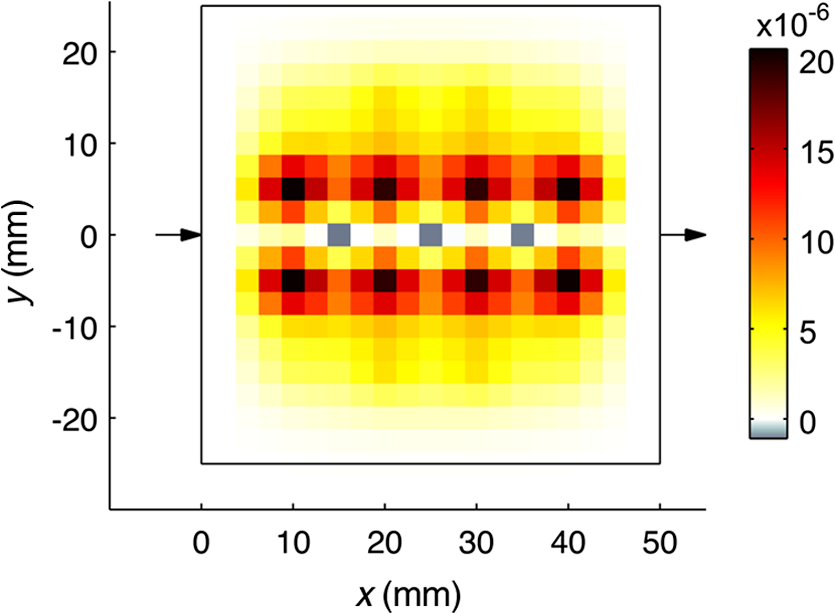
1. Introduction

The purpose of imaging and sensing techniques such as ultrasound-modulated optical tomography (UOT) is the production of images or spatially defined quantitative measurements of some parameter of interest. In the field of optical biomedical imaging, this is typically an image of the optical absorption coefficient within a diffuse medium at a particular wavelength. When multiple wavelengths are employed, the data may be combined via knowledge of the absorption spectra of various chromophores to form physiologically relevant images of, for example, oxygen saturation.

1.1.

Sensitivity and Image Reconstruction in UOT

In UOT, the sensitivity of the system is defined approximately by the product of the optical sensitivity and acoustic amplitude in the system. The vastly different spatial resolutions of the acoustic and diffuse optical aspects of UOT encourage various approaches to the generation of images or spatially localized measurements, depending upon the nature of the optical configuration and the applied acoustic modulation.

The most basic approach is that of direct mapping; when the measurement inherently posses sufficient and controllable spatial selectivity, a measured datum may be assigned directly to the region of assumed sensitivity in an image. This approach is common in systems where the energy that is used to probe the system travels in straight lines without significant diffuse reflection from the interfaces or multiple scattering by a participating medium, such as in X-ray or ultrasound imaging. In a sensing application, the “image” is essentially a single region, but the implicit assumption of spatial resolution remains. Depending upon the application, the spatial resolution afforded by a focused or time gated ultrasound field is arguably sufficient to delineate regions of biological interest. If we neglect acoustic absorption and assume a constant ultrasound excitation amplitude probes each region in a given experiment, a UOT image produced via direct mapping records the scaled optical sensitivity in the medium.¹

In transmission mode configurations of a UOT experiment with a large optical étendue (such as those employing photo-refractive,²^–⁴ photo-refractive polymer,⁵ spectral-hole burning,⁶ CCD,⁷ digital holography,⁸ or speckle contrast⁹ based detection mechanisms) the optical sensitivity through a homogeneous medium transverse to the optical axis is relatively constant when contrasted with the exponentially varying sensitivity parallel to the axis of light collection. Since optical absorbers embedded in a turbid region reduce the optical sensitivity of the system in their vicinity, a transverse scan of the ultrasound probe can provide useful images of the embedded absorbers. Few demonstrations have been provided of more complicated absorption patterns in which shadowing of the optical sensitivity may distort the image, or of systems where an image is generated by a scan parallel to the optical axis in a high étendue system.

In low étendue systems that employ point-like source and/or detection mechanisms, the optical sensitivity varies significantly throughout the image in all optical configurations and scan directions irrespective of the homogeneity of the medium. In the context of UOT, this point was highlighted succinctly by the images produced by Lev and Sfez.¹^,¹⁰ In this case, and in that of a high étendue system with the significant heterogeneity, the fundamental problem is that the optical sensitivity of the system is not uniform.

In the case of pure diffuse optical tomography (DOT), it is the very nonuniformity of the optical sensitivity which is used to generate images of the optical absorption. In DOT, it is recognized that the spatial resolution for a pair of point-like optical source and the detector is unsuitable for the direct image reconstruction, and instead a model-based inversion procedure is employed. In the most general sense, this approach employs a forward model to predict the spatial sensitivity of the measurement and this is used to drive the update of an image based upon the measured data. The DOT problem remains ill-posed, and a-priori information regarding the solution is typically imposed to constrain the reconstruction.

Bratchenia et al.¹¹ previously demonstrated the recovery of the optical absorption coefficient in a turbid medium via a model-based inversion. In their work, the UOT signal was described in the frequency domain, and the acoustically driven modulation of the coherent input light was linearized in a diffusion-style model, similar to that presented by Allmaras and Bangerth.¹² A three-dimensional recovery of the optical absorption coefficient was performed using an iterative nonlinear optimization employing the Levenberg–Marquardt algorithm.

In this work, we take an alternative approach. We employ a time-domain model of the UOT signal which naturally provides many of the oft-employed measurement types in UOT, such as the modulation depth. Our forward model considers the nonlinearity of the acoustically driven decorrelation of the optical field, which allows us to examine in greater depth the form of the sensitivity functions which arise in the UOT experiment. In an approach common in DOT, we linearize our forward model in the optical parameters; this leads to a one-step difference data reconstruction which resolves an absorption perturbation from an assumed known background.

This work specifically considers the case of single fiber point-source and point-detector measurements of the field autocorrelation under monochromatic acoustic excitation.

2. Theory

2.1.

Autocorrelation Measurement in UOT

In an autocorrelation-based UOT experiment, we measure the lag ( $τ$ ) dependent autocorrelation of the flux exiting the medium at a particular location ( $r$ ) on the boundary, $y (r, τ)$ , $r \in δ Ω$ in response to the insonification of the coherently illuminated medium. In practice, this value must be derived from the intensity autocorrelation function via the Seigert relation.¹³ Neglecting an exponential decay in the correlation function due to Brownian motion, the data contain an oscillatory component at the acoustic frequency and its harmonics; this is depicted in Fig. 1. In this work, we consider ultrasound pressures of amplitudes small enough to ensure that only the fundamental frequency is significant; more details of the assumptions employed are presented later when we consider the forward model in Sec. 2.3.

Fig. 1

Illustration of the form of the measurement in autocorrelation ultrasound-modulated optical tomography (UOT). The DC and AC measurement types are found from the nondecaying autocorrelation flux measured on the boundary of a static medium (black line). A fitting algorithm must be used in the case of measurements in a fluid exhibiting decorrelation due to Brownian motion (gray line).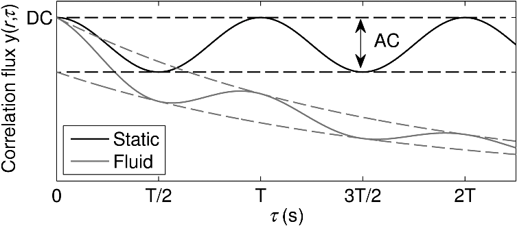

We consider three measurement types:

1. $y {(r)}^{DC} = y (r, 0)$ is equal to the continuous wave (CW or DC) intensity in DOT.
2. $y {(r)}^{AC} = y (r, 0) - y (r, T / 2)$ is the maximum variation, or AC component, of the correlation flux over an acoustic cycle of length $T$ .
3. $m (r) = 1 - y (r, T / 2) / y (r, 0)$ is the modulation depth flux, which is defined as the quotient of the previous two quantities.

2.2.

Linear Image Reconstruction

In this work, we will employ a linear (difference data) reconstruction technique. Although strictly limited to the recovery of qualitative information,¹⁴ its simple formulation allows us to investigate many basic aspects of the UOT inversion, including its sensitivity to noise, and the effects of the a-priori information required to circumvent the ill-posedness of the underlying problem.

Consider a turbid medium parameterized by its spatially varying absorption coefficient, $x (r) = μ_{a} (r)$ . The measured data $y (r, τ)$ are found by the application of the nonlinear operator $F$

Eq. (1)

y (r, τ) = F (τ) [x (r)] .

The operator $F$ incorporates the physics of the problem under the given parameterization, the boundary conditions, a given set of optical sources and detectors, and a particular ultrasound configuration.

In a linear reconstruction, we typically consider the change in a measurement $Δ y = y (r, τ) - y_{0} (r, τ)$ brought about by a perturbation in the parameters $Δ x (r) = x (r) - x_{0} (r)$ . Expanding Eq. (1) in a Taylor series around $x_{0}$ and dropping the spatial and lag dependent notation momentarily

Eq. (2)

y = y_{0} + F^{'} [x_{0}] (x - x_{0}) + \frac{1}{2} {(x - x_{0})}^{T} F^{''} [x_{0}] (x - x_{0}) + \dots,

and then discounting the higher-order terms and rearranging, we get

Eq. (3)

Δ x (r) \approx {(F {(τ)}^{'} [x_{0}])}^{- 1} Δ y (r, τ) .

$F^{'}$ is the first-order Frećhet derivative of the forward model.¹⁵ In the case of the modulation depth measurement

Eq. (4)

m (r) = \frac{y {(r)}^{AC}}{y {(r)}^{DC}} = 1 - \frac{F (T / 2) [x (r)]}{F (0) [x (r)]} .

Expanding this expression in a series around a baseline $x_{0}$ , discounting higher-order terms and rearranging

Eq. (5)

Δ x (r) = - Δ m (r) \times {[\frac{y_{0} {(r)}^{DC} F {(T / 2)}^{'} [x_{0}] - y_{0} {(r)}^{AC} F {(0)}^{'} [x_{0}]}{{[y_{0} {(r)}^{DC}]}^{2}}]}^{- 1} .

Our task in this work is thus to develop an expression for $F^{'}$ . In this work, we will develop the discrete form of this operator which is the Jacobian matrix, $J$ .¹⁶ The inversion procedure of Eq. (3) (or its equivalent modulation depth formulation) is then given by

Eq. (6)

Δ x_{k} = {(J (τ) {[x_{0}]}_{m k})}^{- 1} Δ y_{m} .

2.3.

Forward Model

Sakadžić and Wang¹⁷ previously derived a transport equation which describes the propagation of correlation in a turbid medium under insonification by a monochromatic acoustic field. The authors state a diffusion approximation to this transport equation which is valid under a number of assumptions regarding the nature of the acoustic excitation and optical properties. The principle limitation is that phase increments accrued at successive scattering sites are uncorrelated which requires that $(k_{a} l_{tr}) ≫ 1$ , where $(k_{a} l_{tr})$ is the product of the acoustic wavenumber and the optical transport mean free path $μ_{s}^{' - 1}$ . Other limitations, such as the maximum permissible acoustic pressure amplitude, are introduced by the convenient approximations in the derivation. A more detailed analysis of the requisite approximations is presented in the original work, where the model is experimentally validated, demonstrating a good agreement in the region of validity of the standard optical diffusion approximation. The diffusion approximation reads

Eq. (7)

[- \nabla \cdot κ \nabla + μ_{a} + μ_{s}^{'} h (τ)] G (r, τ) = q_{0} (r, τ), r \in Ω,

where

Eq. (8)

h (τ) = {[P_{0} (r) k_{0} n_{0} / (k_{a} ρ v_{a}^{2})]}^{2} [1 - \cos (ω_{a} τ)] \times [η^{2} (k_{a} l_{tr}) \arctan (k_{a} l_{tr}) + S_{a}^{2} / 3 - 2 η S_{a} \cos (φ_{a})],

where

κ = {(3 μ_{s}^{'})}^{- 1}

is the diffusion coefficient,

μ_{s}^{'} = μ_{s} (1 - g)

is the reduced scattering coefficient,

g

is the scattering anisotropy,

G (r, τ)

is the correlation fluence in the medium,

q_{0}

is an isotropic source term,

P_{0}

is the pressure amplitude of the acoustic field,

k_{0}

is the optical wavenumber in vacuo,

n_{0}

is the refractive index of the medium,

k_{a}

is the acoustic wavenumber,

ρ

is the density of the medium,

v_{a}

is the speed of sound in the medium,

ω_{a}

is the angular acoustic frequency,

η

is the acousto-optic coefficient,

S_{a}

is the amplitude of scatterer displacement relative to the acoustic field, and

ϕ_{a}

is the relative phase of scatterer motion to the acoustic field.

The term $h (r)$ , proportional to the square of the acoustic pressure amplitude, describes the acoustically driven decorrelation of the optical field. For a given medium, and within the region of validity of the model (where $k_{a} l_{tr} ≫ 1$ ), the term is also dependent upon the square of the acousto-optic coefficient (which takes a value of $η \approx 0.32$ in water¹⁸), the square of the optical wavenumber, and has an approximately inverse relationship to the acoustic frequency. The effect of this term is considered for a wide range of $(k_{a} l_{tr})$ in Ref. 19.

This correlation diffusion approximation was originally derived under the conditions of isotropic scattering where $g = 0$ , though it was demonstrated to provide a fair approximation under the replacement of $μ_{s}$ with $μ_{s}^{'}$ .

2.3.1.

Sources, boundary conditions and detectors

A collimated source of coherent light is approximated by an isotropic point source located at a depth $1 / μ_{s}^{'}$ below the incident surface. We employ a modified Robin boundary condition

Eq. (9)

G (r, τ) + 2 A \hat{n} \cdot κ \nabla G (r, τ) = 0, r \in δ Ω,

where

\hat{n}

is the outward normal to the boundary at

r

, and

A

depends upon the refractive index mismatch across the boundary.²⁰ The outgoing correlation flux is given by

Eq. (10)

y (r, τ) = - n \cdot κ \nabla G (r, τ), r \in δ Ω .

In the case of an indexed matched boundary where $A = 1$ , Eqs. (9) and (10) may be combined to give

Eq. (11)

y (r, τ) = \frac{1}{2} G (r, τ), r \in δ Ω, A = 1 .

2.3.2.

Finite-element implementation

We solve the correlation diffusion equation by the finite element method.²¹^–²³ Equation (7) is multiplied by a test function which obeys the boundary conditions, and whose zeroth and first derivatives are integrable over the domain. The boundary conditions of Eq. (9) are incorporated by the subsequent integration by parts. The domain is subdivided into a mesh of nonoverlapping elements joined at $N$ vertex nodes. On this mesh, we define a set of piecewise linear basis functions such that $u_{i} (r_{j}) = δ_{i j}$ for $i, j = 1, \dots, N$ where $r_{j}$ located at the $j$ ’th vertex node. We subsequently approximate the solution $G (r, τ) \approx \sum_{j}^{N} u_{j} (r) G_{j} (τ)$ . Selecting the basis functions in the weak formulation to be the same as the mesh basis allows us to write the resulting linear system of equations:

Eq. (12)

A (τ) [x] G (τ) = q,

where

A

is the finite element system matrix. We express the parameters of the forward model,

x (r)

, the absorption-like decorrelation function

h (r)

, and the diffusion coefficient

κ

using the same basis functions such that, for example,

μ_{a} (r) = \sum_{k} u_{μ, k} (r) μ_{a, k}

. Consequently,

Eq. (13)

A (τ) {[x]}_{i j} = \int_{Ω} \sum_{k} [u_{κ, k} (r) κ_{k} \nabla u_{i} (r) \cdot \nabla u_{j} (r) + [u_{μ, k} (r) μ_{a, k} + u_{h, k} (r) h_{k} (τ)] u_{i} (r) u_{j} (r)] d^{n} r + \frac{1}{2 A} \int_{δ Ω} u_{i} (r) u_{j} (r) d^{n - 1} r .

and

Eq. (14)

q_{j} = \int_{Ω} q_{j} u_{j} (r) d^{n} r .

To make a measurement at a point $r_{i}$ Eq. (11) is implemented by a linear operator $D^{T}$ in which the appropriate elements of the row vector are initialized: $D_{j}^{T} = 1 / 2 u_{j} (r_{i})$ . We may now express a single measurement of Eq. (1) in a discrete form

Eq. (15)

y {(τ)}_{m} = F (τ) {[x]}_{m} = D_{m}^{T} A (τ) {[x]}_{m}^{- 1} q_{m} .

The subscript $m$ indicates that this expression considers a single UOT measurement involving one source location $r_{j, m}$ , one detector location $r_{i, m}$ , and a single ultrasound pressure distribution $p {(r, τ)}_{m}$ . For a single measurement, the linear inversion of Eq. (3) may thus be written

Eq. (16)

Δ x \approx {[{(D_{m}^{T} A (τ) {[x_{0}]}_{m}^{- 1} q_{m})}^{'}]}^{- 1} Δ y {(τ)}_{m} .

2.4.

Correlation Measurement Density Functions and the Jacobian

In Eq. (16), the term ${(D_{m}^{T} A (τ) {[x_{0}]}_{m}^{- 1} q_{m})}^{'}$ represents the sensitivity of the measurement to a perturbation in the parameters of the forward model. In the context of DOT, Arridge generalized such sensitivity functions in the framework of photon-measurement density functions.²²^,²⁴ This work followed earlier derivations of the measurement sensitivity to perturbations in absorption by Schotland et al.,²⁵ who termed this the photon hitting density, and others.²⁶^–²⁸

We now explore the correlation measurement density functions (CMDFs) which arise in correlation-based UOT. We assume that both the scattering coefficient $μ_{s}$ and the acoustic field distribution $p (r, τ)$ does not change between measurement of the baseline and the perturbed state in our linear reconstruction. Assuming that the source term is independent of absorption, we take the derivative of the forward model, expanding the derivative of the inverse system matrix²⁹

Eq. (17)

{(D_{m}^{T} A (τ) {[x_{0}]}_{m}^{- 1} q_{m})}^{'} = - D_{m}^{T} A_{m}^{- 1} {(A (τ) {[x_{0}]}_{m})}^{'} A_{m}^{- 1} q_{m} .

The system is parameterized by only the absorption coefficient of the medium, and we thus take the derivative of the system matrix with respect to each basis coefficient $μ_{a, k}$

Eq. (18)

{(A (τ) {[x_{0}]}_{m})}_{μ_{a, k}}^{'} = \int_{Ω} u_{μ, k} (r) u_{i} (r) u_{j} (r) d r .

We substitute this result back into Eq. (17) which provides an expression for the $k$ ’th element of the $m$ ’th CMDF. By definition, this also defines the $k$ ’th column of the $m$ ’th row of the Jacobian which we seek

Eq. (19)

{(J (τ) {[x_{0}]}_{m}^{T})}_{k} = - D_{m}^{T} A (τ) {[x_{0}]}_{m}^{- 1} {(A (τ) {[x_{0}]}_{m})}_{μ_{a, k}}^{'} A (τ) {[x_{0}]}_{m}^{- 1} q_{m} .

To transform this expression into a more useful form, we exploit the reciprocity of the correlation diffusion equation. Arridge expresses this reciprocity in the context of the diffusion equation³⁰

Eq. (20)

D_{m}^{T} A {[x]}^{- 1} q_{m} = q_{m}^{T} A {[x]}^{- 1} D_{m} .

This expression states that the correlation flux across a point on the boundary of the medium due to an internal source of correlation fluence is equal to the correlation fluence measured at the same point in the medium due to an adjoint source of correlation flux across the same point on the boundary of the medium, when this source is scaled according to the appropriate measurement operator, here $D$ .²⁴ In the discrete case, this reciprocity manifests itself in the symmetry of the finite element system matrix. To proceed, we apply the reciprocity expressed in Eq. (20) to the expression of the Jacobian in Eq. (19)

Eq. (21)

{(J (τ) {[x_{0}]}_{m}^{T})}_{k} = - {(A (τ) {[x_{0}]}_{m}^{- 1} q_{m})}^{T} {(A (τ) {[x_{0}]}_{m})}_{μ_{a, k}}^{'} A (τ) {[x_{0}]}_{m}^{- 1} D_{m},

where we have exploited the symmetry of the system matrix, its inverse and derivatives, and the properties of the transpose operation. Finally, we denote the solution to the forward problem

G {(τ)}_{f, m} = A (τ) {[x_{0}]}_{m}^{- 1} q_{m}

, and the solution to the adjoint problem (in which the source term is the measurement operator)

G {(τ)}_{a, m} = A (τ) {[x_{0}]}_{m}^{- 1} D_{m}

. Thus,

Eq. (22)

{(J (τ) {[x]}_{m}^{T})}_{k} = - G {(τ)}_{f, m}^{T} {(A (τ) {[x_{0}]}_{m})}_{μ_{a, k}}^{'} G {(τ)}_{a, m} .

Here, we see that the Jacobian for a perturbation of absorption in the

k

’th node can be found by taking the inner product of the correlation fluence in the domain due to the (standard) source term, with the product of the basis function derivative term and the correlation fluence in the domain due to the adjoint source. We may thus compute the CMDF for a given ultrasound configuration by two computations of the forward model.

2.4.1.

Modulation depth CMDFs and Jacobian

The CMDFs and Jacobian for the DC measurement type are given directly by Eq. (22). The AC sensitivity functions are straightforward

Eq. (23)

{(J^{AC} {[x]}_{m}^{T})}_{k} = {(J (0) {[x]}_{m}^{T})}_{k} - {(J (T / 2) {[x]}_{m}^{T})}_{k},

and the modulation depth sensitivity functions are given by substituting the two expressions into Eq. (5), as follows:

Eq. (24)

{(J^{MD} {[x]}_{m}^{T})}_{k} = - \frac{y_{0, m}^{DC} {(J (T / 2) {[x]}_{m}^{T})}_{k} - y_{0, m}^{AC} {(J (0) {[x]}_{m}^{T})}_{k}}{{[y_{0, m}^{DC}]}^{2}} .

2.5.

Regularization

Although we expect an improvement in the localization of our UOT sensitivity functions over that of pure DOT, our present model still describes a diffusion process: thus the problem of reconstructing an internal parameter distribution from the data measured on the boundary remains ill-posed, and effectively underdetermined. The consequence of these considerations is that even if the sufficient measurements were available to form a square Jacobian, direct solution of Eq. (6) would fail to produce a stable solution, as noise in the measurements amplifies high-frequency oscillations in the resultant reconstruction.

In order to seek a useful and stable solution, it is conventional to apply some form of regularization to the problem. One commonly employed approach is to make the assumption that a “good” solution is one which balances the norm of the residual $‖ (J (τ) [x_{0}]) Δ x_{g} - Δ y ‖$ with the norm of the solution $‖ Δ x_{g} ‖$ , or its derivatives. This approach is that of the general form of Tikhonov regularization in which we replace the matrix Eq. (6) with a minimization problem

Eq. (25)

Δ x_{g} = \underset{x}{\arg \min} ({‖ J (τ) [x_{0}] Δ y - Δ x ‖}_{2}^{2} + λ^{2} {‖ Δ x ‖}_{2}^{2}) .

For the underdetermined case, this minimization procedure is equivalent to solving³¹

Eq. (26)

Δ x_{g} = {(J (τ) {[x_{0}]}^{T} J (τ) [x_{0}] + λ^{2} L)}^{- 1} J (τ) {[x_{0}]}^{T} Δ y .

In the following section, we employ zeroth-order Tikhonov regularization such that $L = I$ . We select the regularization parameter $λ$ according to the l-curve method, though the point of maximum curvature was chosen by the inspection when the algorithm failed to find the correct point.

3. Results

3.1.

Correlation Measurement Density Functions

In Sec. 2.4, we derived the CMDFs for the three measurement types introduced in Sec. 2.1. We will now visually inspect these sensitivity functions to gain insight into the sensitivity and spatial localization offered by these measurements.

A two-dimensional square domain of side 50 mm is located with its bottom left corner at $(0, - 25) mm$ . The domain is assigned a uniform absorption coefficient $μ_{a} = 0.01 {mm}^{- 1}$ , reduced scattering coefficient $μ_{s}^{'} = 1 {mm}^{- 1}$ , and isotropic scattering $g = 0$ . The refractive index of the domain is 1.4 and a matched boundary is employed. An ultrasonic field with a Gaussian profile of full width half maximum 2 mm and peak amplitude of 0.5 MPa is projected through the plane. An isotropic point source is placed at position (1,0) mm to approximate a collimated source incident perpendicular to the boundary at (0,0). A diffuse detector is located at (50,0) mm and integrates the outgoing flux according to a Gaussian profile with the full width half maximum of 0.1 mm.

Figure 2(a) depicts the zero-lag (intensity) sensitivity function for a given measurement. The approximated collimated source is indicated with the inward arrow at the appropriate location, and the center of the diffuse detector with the outward arrow. This figure demonstrates the characteristic absorption sensitivity profile often seen in the literature of DOT.²⁴^–²⁶ The scale of the linear plot is truncated in the positive direction; regions close to the source and detector demonstrate extremely high sensitivity to absorption perturbations. This sensitivity function is insensitive to the acoustic field location: each row of the DC Jacobian which corresponds to a particular optical source and detector pair will be identical. Since in this work we consider only one such pair, a reconstruction using this information can only result in a scaled and regularized image of the same form as the sole unique sensitivity function depicted in Fig. 2(a). To produce a more detailed image would require that many more optical sources and detectors be employed.

The AC measurement absorption sensitivity is presented in Fig. 2(b). In this image, the acoustic field is scanned to a location of (20,10) mm, as indicated by the crossed circle. This figure demonstrates significant sensitivity in the region of the ultrasound, however, the region of sensitivity extends outward from the insonified region toward the source and detector locations.

Fig. 2

UOT absorption sensitivity functions for a transmission mode measurement with 5 cm source-detector spacing in a two-dimensional square domain 50 mm on a side. The crossed circle at (20,10) mm indicates the acoustic focus. (a) DC correlation measurement density functions (CMDF): $- J (0) {[x_{0}]}_{k}^{T}$ ( ${W m}^{- 1}$ ). (b) AC CMDF: $- (J (0) {[x_{0}]}_{k}^{T} - J (T / 2) {[x_{0}]}_{k}^{T})$ ( ${W m}^{- 1}$ ). (c) MD CMDF: $- J^{MD} {[x_{0}]}_{k}^{T}$ ( $m^{- 1}$ ).

Figure 2(c) demonstrates the modulation depth sensitivity with the acoustic field scanned to the same location, (20,10) mm. This figure demonstrates that measurement type is insensitive to perturbations close to the source, detector, and on a smooth line connecting the two. Placing an optical absorber along this path of insensitivity will reduce the amount of correlated and uncorrelated light reaching the detector by an equal amount such that while the overall light level falls, the modulation depth remains constant. This argument is clearly supported by the analytical form of the sensitivity function given in Eq. (4).

The modulation depth sensitivity functions demonstrate high sensitivity in the region of the applied acoustic field. Moving away from the acoustic focus, across the path of zero sensitivity, we encounter a region of negative sensitivity where a perturbation in absorption will attenuate more correlated light than uncorrelated light.

In Fig. 3, we demonstrate the modulation depth sensitivity as we scan the acoustic field through the medium, with the same color scale as Fig. 2(c). Note in particular that when the acoustic field is focused in the region of greatest optical sensitivity (as seen in the DC sensitivity of Fig. 2(a)), the sensitivity function appears to have the highest spatial localization, with two regions of negative sensitivity appearing in the profile. This may be problematic in a direct mapping approach as the absorption perturbations will be averaged over the entire region of sensitivity, but is automatically accounted for in the image reconstruction process.

Fig. 3

Nine UOT MD CMDFs for various ultrasound scan locations which form part of the full MD Jacobian employed in the reconstructions of Fig. 6. Color scale as per Fig. 2(c).

3.2.

Linear Reconstruction: Noise, Regularization, and Comparison With Direct Mapping

Having examined the form of the individual CMDFs which together form the Jacobian, we reconstruct an image under varying degrees of noise. The purpose of this exercise is twofold: first, the procedure will evaluate the functioning of the reconstruction process; second, the regularization required as a function of noise will be assessed. We perform the reconstruction on both the AC and modulation depth measurements.

The reconstruction is performed on an homogeneous background with a regular set of absorption perturbations such that any aberrations in the reconstructed image will be evident. The background domain is the same as employed in Sec. 3.1. The perturbation domain is formed by adding an array of 16 circular perturbations of radius 2.5 mm with a modified absorption coefficient of $0.02 {mm}^{- 1}$ . The perturbed measurements were generated using an independent mesh from the background measurements in order to prevent committing the inverse crime of generating measurements by the same model by which they are inverted.³² To demonstrate an “ideal” reconstruction, the perturbed absorption coefficient was interpolated from its mesh to the baseline mesh upon which the Jacobian is computed, and the resultant image is displayed in Fig. 4.

Fig. 4

Absorption perturbation $Δ μ_{a}$ [ ${mm}^{- 1}$ ] interpolated from the perturbation mesh to the baseline mesh upon which the Jacobian is computed. The baseline mesh does not include features of the perturbed geometry and hence the boundaries are seen to be slightly blurred.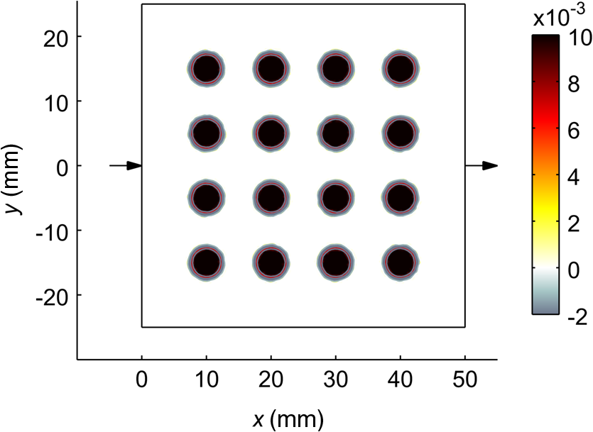

The measurement set was generated by scanning an ultrasonic field with a Gaussian profile of full width half maximum 2 mm and peak amplitude of 0.5 MPa through the domain from $(5, - 25)$ to (45,25) mm at 0.5 mm increments in the $x$ and $y$ . This resulted in a total of $17 \times 21 = 357$ measurements for both the baseline and perturbed measurement.

Figure 5(a) shows a noise-free reconstruction using the AC measurement type. This provides a reasonable qualitative reconstruction of the absorption perturbations of Fig. 4. This is especially true when it is considered that the square region enclosing each absorption perturbation is, in the ideal case, sampled by only 25 ultrasound scan locations. We note, however, that there are large aberrations near the source and detector where the AC CMDFs demonstrate considerable sensitivity. As shown in Fig. 5(b), adding 0.5% of proportional Gaussian noise degrades the reconstruction to the point where the perturbations are just recognizable. The increased regularization required to reconstruct this image has also suppressed the aberrations near to the source and detector.

Fig. 5

Reconstruction of the absorption perturbation, $Δ μ_{a}$ ( ${mm}^{- 1}$ ), depicted in Fig. 4 using the UOT AC measurements under the addition of varying amounts of proportional Gaussian noise. (a) 0% noise and (b) 0.5% noise.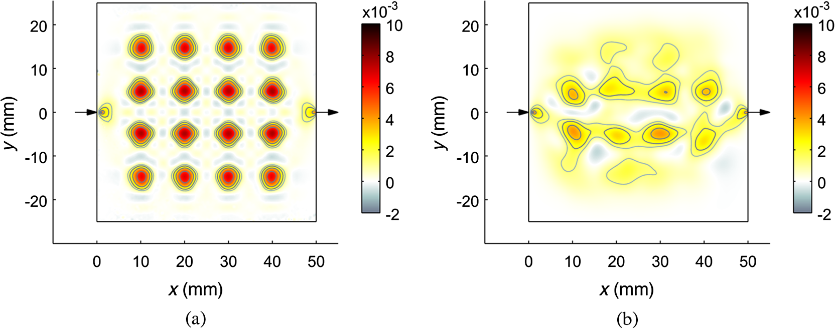

The reconstructions of Fig. 6 demonstrates the modulation depth reconstruction in the case of measurements without noise, with 0.5%, and 1% Gaussian noise. In the noise-free reconstruction, an excellent approximation to the actual perturbation is generated both in a qualitative and quantitative sense. As suggested by the CMDFs displayed previously, the source and detector locations are completely suppressed in the resultant images. As the level of noise in the image is increased, the sensitivity off-axis is gradually suppressed by regularization. In the case of 1% noise, only those perturbations directly on on-axis are perceivable, though this measurement type appears to perform better than the equivalent AC reconstructions.

Fig. 6

Reconstruction of the absorption perturbation, $Δ μ_{a}$ ( ${mm}^{- 1}$ ), depicted in Fig. 4 using the UOT modulation depth measurements under the addition of varying amounts of proportional Gaussian noise. (a) 0% noise, (b) 0.5% noise, and (c) 1% noise.

To demonstrate the improvement of the reconstructed images over that of a direct mapping approach, Fig. 7 illustrates the image formed by directly assigning the modulation depth difference measurement, $Δ m (r)$ , to pixels located at the centers of the acoustic foci. In the absence of noise, the absorption perturbations along the axis of optical sensitivity (Fig. 2(a)) can be distinctly located. The direct mapping approach demonstrates similar spatial resolution to the reconstructed images: this is to be expected since the sensitivity of the modulation depth measurement was previously demonstrated to be highly localized to the region of the acoustic focus. Without compensating for the spatially varying optical sensitivity, those absorbers off-axis are imperceptible. Moreover, the resulting unit-less image provides no quantitative information as would be required if we wished to attempt a recovery of a clinically relevant parameter. It is a common feature of many hybrid imaging modalities that the relationship of the data to the desired parameter is often unclear. We also note that in the case of image reconstruction, a variety of rigorous regularization strategies can be applied to stabilize the recovery of the underlying parameters under varying degrees of noise. In a direct mapping experiment, we may attempt to reduce the deleterious effects of the noise by some form of spatial filtering (for example, convolution with a smoothing kernel), but any such approach is somewhat ad-hoc.

Fig. 7

Modulation depth direct mapping image of the absorption perturbations depicted in Fig. 4.

4. Discussion and Conclusions

The sensitivity functions and associated reconstructed images presented in this work provide considerable insight into the potential of autocorrelation-based UOT. It has been shown that by moving the focus of an acoustic field in the medium, additional spatial resolution can be introduced into the UOT reconstruction: in the case of CW DOT, this would require that additional optical sources and detectors were employed, with associated cost and complexity.

Reconstructions based directly upon the AC measurement type are, in the absence of noise, capable of reproducing a fair representation of the underlying absorption perturbations. A disadvantage of this measurement type is the significant erroneous absorption indicated near the source and detector positions: this is a direct consequence of the extreme sensitivity of the measurement in these regions. If an absorption perturbation were placed near the source or detector, the influence of this measurement change would dominate the resulting image.

In a reconstruction employing both the AC and DC measurements, regularization would suppress the contributions from the AC measurements in which the perturbation from the DC value is below the noise floor. In this sense, the enhancement of a DOT imaging system with ultrasound-modulated correlation measurements will lead to a worse-case imaging resolution equivalent to that of CW DOT, with improved ultrasound-modulated resolution where the noise permits. The influence of the high regions of sensitivity near the source and detector remains a problem, however.

In contrast, the modulation depth measurement type completely suppresses sensitivity near the source and detector positions. Furthermore, the image reconstruction process is capable of producing acceptable results at levels of noise higher than in the AC measurement reconstruction. Suppressing sensitivity in regions close to the source and detector may be valuable in biomedical applications where the physiological changes in a superficial region may otherwise dominate the measurement.³³

The amount of noise added to these reconstructions was chosen to explore to the level at which the reconstructed images are degraded to the extent that they no longer provided any qualitatively useful information. In practice, the amounts of noise which can be tolerated will be dependent upon the nature of the illumination, the applied acoustic field, and the magnitude of the absorption perturbation. Some of the consequences of noise are discussed further in the following section.

In summary, we have demonstrated that standard techniques for image reconstruction in DOT can be successfully employed in UOT. The alternative measurement types available in UOT demonstrate sensitivity with a significantly improved spatial resolution over that of continuous-wave DOT. The modulation depth measurement type, and associated sensitivity functions, demonstrate particularly attractive qualities in suppressing the high sensitivity close to the source and detector, while also providing a better noise immunity than the direct use of the AC measurement data.

5. Future Work

The next step in the development of this work is to conduct reconstructions based upon the experimental data. The signal-to-noise ratio for autocorrelation-based experimental data is a direct function of the permissible integration (data collection) time of the autocorrelation function which defines the measurement. Data collected from fluid targets will be corrupted by an exponential decay caused by decorrelation due to the Brownian motion: this will increase the required integration time as the data must be multiplied by the inverse exponential, amplifying noise on the signal. In any case, it is the integration time which will dictate the applicability of this method to real-world problems in biomedical imaging.

Regarding the theoretical development, four points of particular interest for the future studies are immediately identifiable:

1. Extending the parametrization of the medium to include the scattering coefficient within the domain. This may require an analysis of the uniqueness of the inversion process: in the case of DOT, continuous-wave measurements cannot be used to recover both absorption and scattering perturbations³⁴ and it is unclear without further analysis if this is also true of autocorrelation based measurements.
2. Employing a nonlinear inversion for the absolute recovery of the desired parameters. In UOT, forming the Jacobian matrix requires the forward model to be solved twice for each ultrasound location: this is potentially too slow for a standard iterative reconstruction.³⁵ This problem might therefore be approached by a gradient-based method as employed in both DOT (Ref. 36) and quantitative photoacoustic tomography.³⁷ An alternative approach might be the acceleration of the forward model by the approximation of the acoustically generated sink of correlation by a (Born/Rytov) series approach.
3. Further regularization strategies should be explored based upon a-priori information regarding the structure of the object to be imaged. The image reconstructed in this work might be more suitably regularized using, for example, a total-variation technique, which can only be employed in an iterative, nonlinear inversion.
4. To improve the accuracy of the reconstruction, irrespective of the particular regularization or inversion procedure, a higher quality forward model could be employed. Recent advances in GPU accelerated Monte-Carlo techniques for UOT offer one option.³⁸^,³⁹ This could alternatively be approached by the application of an order-of-scattering approach to the integral form of a correlation transport equation, as employed in DOT⁴⁰.

Acknowledgments

The authors would like to thank Simon Arridge, Ben Cox, Jem Hebden, Emma Malone, and Sava Sakadžić for their advice and support. This work was funded by EPSRC Grant No. EP/G005036/1.

References

1.

A. LevB. G. Sfez, “Pulsed ultrasound-modulated light tomography,” Opt. Lett., 28 (17), 1549 –1551 (2003). http://dx.doi.org/10.1364/OL.28.001549 OPLEDP 0146-9592 Google Scholar

2.

F. Ramazet al., “Photorefractive detection of tagged photons in ultrasound modulated optical tomography of thick biological tissues,” Opt. Express, 12 (22), 5469 –5474 (2004). http://dx.doi.org/10.1364/OPEX.12.005469 OPEXFF 1094-4087 Google Scholar

3.

T. W. Murrayet al., “Detection of ultrasound-modulated photons in diffuse media using the photorefractive effect,” Opt. Lett., 29 (21), 2509 –2511 (2004). http://dx.doi.org/10.1364/OL.29.002509 OPLEDP 0146-9592 Google Scholar

4.

E. Bossyet al., “Fusion of conventional ultrasound imaging and acousto-optic sensing by use of a standard pulsed-ultrasound scanner,” Opt. Lett., 30 (7), 744 –746 (2005). http://dx.doi.org/10.1364/OL.30.000744 OPLEDP 0146-9592 Google Scholar

5.

Y. Suzukiet al., “High-sensitivity ultrasound-modulated optical tomography with a photorefractive polymer,” Opt. Lett., 38 (6), 899 –901 (2013). http://dx.doi.org/10.1364/OL.38.000899 OPLEDP 0146-9592 Google Scholar

6.

Y. Liet al., “Pulsed ultrasound-modulated optical tomography using spectral-hole burning as a narrowband spectral filter,” Appl. Phys. Lett., 93 (1), 11111 (2008). http://dx.doi.org/10.1063/1.2952489 APPLAB 0003-6951 Google Scholar

7.

S. Lévêqueet al., “Ultrasonic tagging of photon paths in scattering media: parallel speckle modulation processing,” Opt. Lett., 24 (3), 181 –183 (1999). http://dx.doi.org/10.1364/OL.24.000181 OPLEDP 0146-9592 Google Scholar

8.

M. GrossP. GoyM. Al-Koussa, “Shot-noise detection of ultrasound-tagged photons in ultrasound-modulated optical imaging,” Opt. Lett., 28 (24), 2482 –2484 (2003). http://dx.doi.org/10.1364/OL.28.002482 OPLEDP 0146-9592 Google Scholar

9.

J. LiG. KuL. V. Wang, “Ultrasound-modulated optical tomography of biological tissue by use of contrast of laser speckles,” Appl. Opt., 41 (28), 6030 –6035 (2002). http://dx.doi.org/10.1364/AO.41.006030 APOPAI 0003-6935 Google Scholar

10.

A. LevB. G. Sfez, “Direct, noninvasive detection of photon density in turbid media,” Opt. Lett., 27 (7), 473 (2002). http://dx.doi.org/10.1364/OL.27.000473 OPLEDP 0146-9592 Google Scholar

11.

A. Bratcheniaet al., “Acousto-optic-assisted diffuse optical tomography,” Opt. Lett., 36 (9), 1539 (2011). http://dx.doi.org/10.1364/OL.36.001539 OPLEDP 0146-9592 Google Scholar

12.

M. AllmarasW. Bangerth, “Reconstructions in ultrasound modulated optical tomography,” J. Inverse Ill-posed Probl., 19 (6), 801 –823 (2011). http://dx.doi.org/10.1515/jiip.2011.050 0928-0219 Google Scholar

13.

B. J. BerneR. Pecora, Dynamic Light Scattering, With Applications to Chemistry, Biology, and Physics, Courier Dover Publications(2000). Google Scholar

14.

D. Boas, “A fundamental limitation of linearized algorithms for diffuse optical tomography,” Opt. Express, 1 (13), 404 (1997). http://dx.doi.org/10.1364/OE.1.000404 OPEXFF 1094-4087 Google Scholar

15.

S. R. ArridgeJ. C. Schotland, “Optical tomography: forward and inverse problems,” Inverse Probl., 25 (12), 123010 (2009). http://dx.doi.org/10.1088/0266-5611/25/12/123010 INPEEY 0266-5611 Google Scholar

16.

S. R. ArridgeM. Schweiger, “Image reconstruction in optical tomography,” Philos. Trans. R. Soc. B, 352 (1354), 717 –726 (1997). http://dx.doi.org/10.1098/rstb.1997.0054 PTRBAE 0962-8436 Google Scholar

17.

S. SakadžićL. V. Wang, “Correlation transfer and diffusion of ultrasound-modulated multiply scattered light,” Phys. Rev. Lett., 96 (16), 163902 (2006). http://dx.doi.org/10.1103/PhysRevLett.96.163902 PRLTAO 0031-9007 Google Scholar

18.

V. RamanK. S. Venkataraman, “Determination of the adiabatic piezo-optic coefficient of liquids,” Proc. R. Soc. London, Ser. A, 171 (945), 137 –147 (1939). http://dx.doi.org/10.1098/rspa.1939.0058 PRLAAZ 0080-4630 Google Scholar

19.

S. SakadžićL. V. Wang, “Modulation of multiply scattered coherent light by ultrasonic pulses: an analytical model,” Phys. Rev. E, 72 (3), 036620 (2005). http://dx.doi.org/10.1103/PhysRevE.72.036620 PLEEE8 1063-651X Google Scholar

20.

M. Schweigeret al., “The finite element method for the propagation of light in scattering media: boundary and source conditions,” Med. Phys., 22 (11), 1779 –1792 (1995). http://dx.doi.org/10.1118/1.597634 MPHYA6 0094-2405 Google Scholar

21.

S. R. Arridge, “A finite element approach for modeling photon transport in tissue,” Med. Phys., 20 (2), 299 –309 (1993). http://dx.doi.org/10.1118/1.597069 MPHYA6 0094-2405 Google Scholar

22.

S. R. ArridgeM. Schweiger, “Photon-measurement density functions. Part 2: finite-element-method calculations,” Appl. Opt., 34 (34), 8026 –8037 (1995). http://dx.doi.org/10.1364/AO.34.008026 APOPAI 0003-6935 Google Scholar

23.

J. Heinoet al., “Anisotropic effects in highly scattering media,” Phys. Rev. E, 68 (3), 031908 (2003). http://dx.doi.org/10.1103/PhysRevE.68.031908 PLEEE8 1063-651X Google Scholar

24.

S. R. Arridge, “Photon-measurement density functions. Part I: analytical forms,” Appl. Opt., 34 (31), 7395 –7409 (1995). http://dx.doi.org/10.1364/AO.34.007395 APOPAI 0003-6935 Google Scholar

25.

J. C. SchotlandJ. C. HaselgroveJ. S. Leigh, “Photon hitting density,” Appl. Opt., 32 (4), 448 –453 (1993). http://dx.doi.org/10.1364/AO.32.000448 APOPAI 0003-6935 Google Scholar

26.

S. FengF.-A. ZengB. Chance, “Photon migration in the presence of a single defect: a perturbation analysis,” Appl. Opt., 34 (19), 3826 (1995). http://dx.doi.org/10.1364/AO.34.003826 APOPAI 0003-6935 Google Scholar

27.

E. M. Sevicket al., “Localization of absorbers in scattering media by use of frequency-domain measurements of time-dependent photon migration,” Appl. Opt., 33 (16), 3562 (1994). http://dx.doi.org/10.1364/AO.33.003562 APOPAI 0003-6935 Google Scholar

28.

J. Changet al., “Imaging diffusive media using time-independent and time-harmonic sources: dependence of image quality on imaging algorithms, target volume, weight matrix, and view angles,” Proc. SPIE, 2389 448 –464 (1995). http://dx.doi.org/10.1117/12.209995 PSISDG 0277-786X Google Scholar

29.

M. AbramowitzI. A. Stegun, Handbook of Mathematical Functions, With Formulas, Graphs, and Mathematical Tables, Courier Dover Publications(1964). Google Scholar

30.

S. R. Arridge, “Optical tomography in medical imaging,” Inverse Probl., 15 (2), R41 –R93 (1999). http://dx.doi.org/10.1088/0266-5611/15/2/022 INPEEY 0266-5611 Google Scholar

31.

M. BerteroP. Boccacci, Introduction to Inverse Problems in Imaging, Taylor & Francis(2010). Google Scholar

32.

D. L. ColtonR. Kress, Integral Equation Methods in Scattering Theory, Wiley, New York (1983). Google Scholar

33.

I. Tachtsidiset al., “False positives in functional near-infrared topography,” Adv. Exp. Med. Biol., 645 307 –314 (2009). http://dx.doi.org/10.1007/978-0-387-85998-9_46 AEMBAP 0065-2598 Google Scholar

34.

S. R. ArridgeW. R. B. Lionheart, “Nonuniqueness in diffusion-based optical tomography,” Opt. Lett., 23 (11), 882 –884 (1998). http://dx.doi.org/10.1364/OL.23.000882 OPLEDP 0146-9592 Google Scholar

35.

M. SchweigerS. R. ArridgeI. Nissilä, “Gauss–Newton method for image reconstruction in diffuse optical tomography,” Phys. Med. Biol., 50 (10), 2365 –2386 (2005). http://dx.doi.org/10.1088/0031-9155/50/10/013 PHMBA7 0031-9155 Google Scholar

36.

S. R. ArridgeM. Schweiger, “A gradient-based optimisation scheme for optical tomography,” Opt. Express, 2 (6), 213 –226 (1998). http://dx.doi.org/10.1364/OE.2.000213 OPEXFF 1094-4087 Google Scholar

37.

T. Saratoonet al., “A gradient-based method for quantitative photoacoustic tomography using the radiative transfer equation,” Inverse Probl., 29 (7), 075006 (2013). http://dx.doi.org/10.1088/0266-5611/29/7/075006 INPEEY 0266-5611 Google Scholar

38.

T. S. LeungS. Powell, “Fast Monte Carlo simulations of ultrasound-modulated light using a graphics processing unit,” J. Biomed. Opt., 15 (5), 055007 (2010). http://dx.doi.org/10.1117/1.3495729 JBOPFO 1083-3668 Google Scholar

39.

S. PowellT. S. Leung, “Highly parallel Monte-Carlo simulations of the acousto-optic effect in heterogeneous turbid media,” J. Biomed. Opt., 17 (4), 045002 (2012). http://dx.doi.org/10.1117/1.JBO.17.4.045002 JBOPFO 1083-3668 Google Scholar

40.

A. K. Jhaet al., “Simulating photon-transport in uniform media using the radiative transport equation: a study using the Neumann-series approach,” J. Opt. Soc. Am. A, 29 (8), 1741 –1757 (2012). http://dx.doi.org/10.1364/JOSAA.29.001741 JOAOD6 0740-3232 Google Scholar

Biographies of the authors are not available.

CC BY: © The Authors. Published by SPIE under a Creative Commons Attribution 4.0 Unported License. Distribution or reproduction of this work in whole or in part requires full attribution of the original publication, including its DOI.

Citation Download Citation

Samuel Powell and Terence S. Leung "Linear reconstruction of absorption perturbations in coherent ultrasound-modulated optical tomography," Journal of Biomedical Optics 18(12), 126020 (31 December 2013). https://doi.org/10.1117/1.JBO.18.12.126020

Published: 31 December 2013

Access the abstract

JOURNAL ARTICLE
9 PAGES

DOWNLOAD PAPER SAVE TO MY LIBRARY

GET CITATION

CITATIONS

Cited by 7 scholarly publications.

Explore citations on Lens.org

KEYWORDS

Absorption

Ultrasound-modulated optical tomography

Acoustics

Sensors

Modulation

Ultrasonography

Diffusion

1.

Introduction

1.1.

Sensitivity and Image Reconstruction in UOT

2.

Theory

2.1.

Autocorrelation Measurement in UOT

Fig. 1

2.2.

Linear Image Reconstruction

Eq. (1)

Eq. (2)

Eq. (3)

Eq. (4)

Eq. (5)

Eq. (6)

2.3.

Forward Model

Eq. (7)

Eq. (8)

2.3.1.

Sources, boundary conditions and detectors

Eq. (9)

Eq. (10)

Eq. (11)

2.3.2.

Finite-element implementation

Eq. (12)

Eq. (13)

Eq. (14)

Eq. (15)

Eq. (16)

2.4.

Correlation Measurement Density Functions and the Jacobian

Eq. (17)

Eq. (18)

Eq. (19)

Eq. (20)

Eq. (21)

Eq. (22)

2.4.1.

Modulation depth CMDFs and Jacobian

Eq. (23)

Eq. (24)

2.5.

Regularization

Eq. (25)

Eq. (26)

3.

Results

3.1.

Correlation Measurement Density Functions

Fig. 2

Fig. 3

3.2.

Linear Reconstruction: Noise, Regularization, and Comparison With Direct Mapping

Fig. 4

Fig. 5

Fig. 6

Fig. 7

4.

Discussion and Conclusions

5.

Future Work

Acknowledgments

References

Show All Keywords

Keywords/Phrases

Search In:

Publication Years