
|
|
1.IntroductionThis paper presents a novel technique for measuring the fluorescence from individual cells or microspheres in a sample. This technique is widely applicable to cytopathology, the diagnosis of disease based on the analysis of cells in solution. Each year, 1.4 billion cytology samples are processed in clinical laboratories.1 The two most common cytology tests are blood counts and Pap smears,2 but increasingly, cell analysis is also being used to diagnose solid cancer tumors by collecting samples with a fine-needle aspiration biopsy.3 Clinical cytopathology can be performed using either a microscope or a flow cytometer. Microscopes allow the user to view a limited number of static cells in detail. Flow cytometers, in comparison, measure many more cells by quickly analyzing one cell at a time in multiple fluorescence channels. These measurements are presented as histograms or density plots that define distinct cell populations. Flow cytometry measurements are used clinically to diagnose and monitor response to treatment in leukemia, AIDS, and increasingly a variety of solid-tumor cancers.4,5 Commercial flow cytometers are widely used clinically and have even more uses in biological research, but their large size, weight, and cost have driven research to develop miniature alternatives.6 Two approaches have been taken to miniaturize flow cytometers. The first approach uses the same basic design as conventional flow cytometers; the cells or microspheres are formed into a single file line and sensed one at a time. Much of the work in this area has focused on developing methods to accurately position the cells in a line. Many of these instruments have used conventional fluorescence microscopes for sensing.7 The size of these systems has been further reduced by replacing the microscope with a discrete light emitting diode (LED) light source and a discrete photodiode.8 Other groups have built even more compact systems by integrating optical components into the microflow cytometer while continuing to use an external sensor.9 The second approach is to improve the cell analysis rate by using a large number of sensing elements operating in parallel to perform what is called either lensfree or lensless imaging.10,11 Unlike traditional flow cytometers, cells are not forced into a single file line in these systems so even with lower lateral flow rates, many more cells can be analyzed with these systems. Early work in this technique demonstrated the ability to distinguish between up to 100,000 red blood cells, yeast cells, and Escherichia coli cells in a single image.10 Multiple illumination angles were then used to measure the height of cells in shadow imaging.12 More recently the technique has been applied to three-dimensional (3-D) imaging of capillary morphogenesis.13 The work has even been extended to video rate imaging for tracking of human sperm to characterize movement patterns.14,15 Traditionally, the big limitation of these systems has been their ability to only measure cell size and position, not the fluorescence signal used in flow cytometers. Fluorescence imaging is challenging because the fluorescence signal from the sample is weak, the signal from the excitation source must be filtered before recording the emission from the sample, and unlike shadows, fluorescence signals are not directional. These constraints require very low sample-senor separation during lensless fluorescence imaging (LFI). Recently, LFI systems have been presented. Lensfree fluorescence imaging of Caenorhabditis elegans was performed by illuminating a thin layer of the sample using the total internal reflection allowing for detailed imaging.16 Imaging slightly deeper into the sample was performed using time-domain excitation separation using high speed pixels for LFI, but a “flow and stop” protocol was used where the microparticles had to settle to the bottom of the channel prior to sensing for a fixed 20 μm spacing.17 Higher resolution images of fluorescently labeled adherent cells was measured using an interference filter to measure cells that were separated by just 6 μm from the sensor.18 Spatial deconvolution was used to improve the resolution of lensless fluorescence images for a system with fixed sensor-sample separation and external optical components including a fiber optic phase plate and a filter.19 In this work, a simplified lensless fluorescence imager is presented consisting of a single illuminator and imager chip. The concept of spatial deconvolution is extended to samples including fluorophores at various heights. The method is calibrated using the multiangle shadow imaging technique referenced above. Then, LFI is demonstrated on cells flowing through a microfluidic channel. 2.MethodsThis paper demonstrates that fluorescence from cell-sized microspheres and cells can be accurately measured at separations from 5 to 35 μm representing the entire height of a microfluidic channel. Within this range, the height of the microsphere can be calculated by measuring the shape of the measured fluorescence image from each microsphere. This work is divided into two processes. The novel process of fluorescence lensless imaging uses a single illumination source to capture a single image of the fluorescently labeled sample which is then processed to estimate the sample-sensor separation. This method is calibrated and verified using the established method of shadow imaging using the multiple light sources to capture multiple images to calculate the height. Since uniformly labeled fluorescent samples are used in this work, the two methods give comparable results. For the real world samples where the fluorescence intensity is related to a biologically relevant feature of the cell, the fluorescence signal contains more information than the shadow signal. This work is built on seven methods: simulation of the light measured from LFI, imager preparation for LFI, phantom preparation of microspheres at fixed height above the imager, particle height calculation by shadow triangulation, LFI, image processing to calculate particle height from LFI, and finally LFI of flowing cells. 2.1.SimulationFluorophores were modeled as omnidirectional point light sources to perform simulations of fluorescence lensless imaging. As shown in Appendix, a point light source at height, , above the imaging plane casts light of intensity, , at a distance, , from the point on the plane closest to the light source The distribution of fluorophores in a cell or microsphere was modeled by adding the effect of thousands of omnidirectional light sources evenly distributed throughout a unit sphere. The positions of the light sources were determined by superimposing a 3-D grid on top of the sphere. The grid size was chosen so that 10 points were included between the center of the sphere and the edge. A light source was added at each integer point on this grid that fell within the sphere for a total of 4160 points. A MATLAB (MathWorks) script was developed to calculate the illumination pattern for different separations between the sphere and the imager. 2.2.Imager PreparationCommercial imagers are almost universally shipped with cover glass protecting the sensor from moisture, dust, and mechanical interactions. In both conventional imaging applications and lensless shadow imaging, this glass has only minor effects on imaging quality, but for LFI the minimum sample-sensor separation of approximately 1 mm imposed by this cover glass significantly decreases the performance. The cover glass can be attached to the imaging sensor either indirectly by first mounting the sensor in a carrier and then attaching the glass to the carrier or directly by first connecting the glass to the wafer and then cutting the wafer into individual sensors.20 It is very challenging to remove the cover glass without damaging the sensor when it is attached directly. In this work, a variety of commercial imager chips were examined and the packages used in two commercial web cameras (Logitech QuickCam Communicate MP and Logitech QuickCam Pro 9000, New York, California) were determined to be the most easily removed. In these chips, the cover glass is glued to a plastic package that surrounds the imager. The cover glass was removed by first carefully scoring the plastic package along with the edge of the glass using a scalpel and then using the scalpel to lever the glass out. After removing the cover glass, the imager was tested to ensure that it continues to function as designed, but placing a liquid sample directly on the imager resulted in immediate failure. The imager was protected by encapsulating the bond pads and bond wires with cyanoacrylate glue (Scotch Super Glue). The imager was held at an angle so that the glue would flow toward the edge and the glue was dispensed from a syringe (BD Insulin Syringe Ultra-Fine 30 Gauge). The imager was then allowed to cure in an open area to minimize redeposition of glue on the imager surface. 2.3.Phantom PreparationIn order to keep fluorescent microspheres at fixed locations above the imager for shadow and fluorescence imaging, simple phantoms were fabricated using 12 μm fluorescent microspheres (Spherotech FP-10045-2) and agarose (Bioworld Agarose Low Melt Temperature). The microspheres were diluted in deionized water to form a working solution. A 3% solution of the agarose was prepared following the manufacturer’s instructions to mix 90 mg of agarose powder with 3 mL of deionized water. The mixture was then placed in the microwave at high power for 30 s to dissolve the agarose. The melted agarose solution was then kept in a bath of boiling water until used. About 35 μl of the agarose solution was pipetted on top of the imager. About 2 μl of the microsphere solution was then pipetted into the agarose solution as close to the imager as possible. LFI was performed to identify if microspheres had settled. If not, the imager was placed under a heater for approximately 15 s to allow the microspheres to settle. If microspheres had settled, the imager was placed in a freezer for 1 min to set. 2.4.Shadow ImagingThe established technique of shadow imaging was used to calibrate the new LFI technique.12 The height of cells can be determined by using light sources mounted at different angles above the imager. As shown in Fig. 1(a), when the sample is illuminated by a source directly above the imager, a shadow is cast by each microsphere directly below its location. Shifting the light source shifts the shadow. The height of the sample, , can be calculated using the right triangles that are formed as depicted in Fig. 1(b), where is the movement of the sample’s shadow due to the movement of the light source, is the separation between the light source and the sensor, and “” is the lateral displacement of the light source. Fig. 1Diagrams demonstrating shadow imaging. (a) The position of the shadow moves as the light source moves. (b) The height of the sample can be calculated using two shadows cast by the sample from different light sources using the similar triangles shown here.  Rather than moving a single light source, an illuminator was built that contained five LEDs (Lite-On White LED LTW-670DS). Each LED was independently controlled by a microcontroller (Microchip 18F4550) that communicated with a personal computer over the universal serial bus. The LEDs were mounted on a sheet metal box formed in the shape of a trapezoid as shown in Fig. 2. Initial experiments showed that it was difficult to accurately determine the position of the LEDs in a bowl shape and that using a rectangular enclosure resulted in little illumination from the LEDs at the sides reaching the sample because they are pointed in the wrong direction. The trapezoid shape offered a simple geometry while pointing the LEDs close enough to the sample to ensure strong illumination. Images were captured with the CMOS imager for each illumination setting with 5.3 ms exposure time, low gain, and high contrast settings. 2.5.Lensless Fluorescence ImagingThe novel LFI method is divided into two parts: exciting the fluorophores and measuring the light they emit. LFI does not use a filter to block the excitation light from hitting the sensor, so it is important to excite with light that the sensor does not measure. In this work, a handheld 254-nm light (Ultraviolet Products, LLC UVGL-55, Upland, California) was used because CMOS sensors are insensitive to this wavelength. The bulb also emits low levels of visible light, so these wavelengths were filtered out using a bandpass UV filter (Omega Optical, 250BP30, Brattleboro, Vermont). This illuminator is then placed as close to the imager as possible using a styrofoam stand. Emitted photons were captured using a CMOS imager (Quickcam Communicate MP) prepared as described above. In order to capture the relatively faint fluorescence signal, the exposure was set to the maximum value of 1 s, gain was turned up to high, and contrast was turned down to medium. 2.6.Image ProcessingThe images from shadow and fluorescence imaging were processed in MATLAB to generate the calibration graph. This processing took place in two stages. First, the fluorescence image was processed to detect microsphere location and fluorescence shape. Then, the shadow images of the same sample were processed to determine the height of each microsphere. The first step while analyzing the fluorescence image was to determine the approximate center of each microsphere. This process is shown for the simulated data from two microspheres in Fig. 3. First, the image was thresholded to create a black and white image as shown in Fig. 3(a). Noise in the original image can occasionally create a single pixel that is not connected with the other pixels representing a microsphere, so the thresholded image was then dilated by expanding each white pixel by two pixels in every direction to form the image in Fig. 3(b). Each connected region of white pixels was then given a region number shown as different colors in Fig. 3(c). The center of each region, marked with an “” in Fig. 3(d), was calculated by averaging the coordinates of all the pixels in that region. This location was used as an initial estimate of the center of the microsphere, but it was often inaccurate because the thresholding process was very sensitive to noise. Fig. 3The approximate location of the center of each fluorescent microsphere is located in four steps. (a) Raw data are thresholded. (b) The image is dilated so that each sphere is represented by a single contiguous region. (c) Each region is numbered. (d) The center of each region is identified by averaging the pixel values in that region. 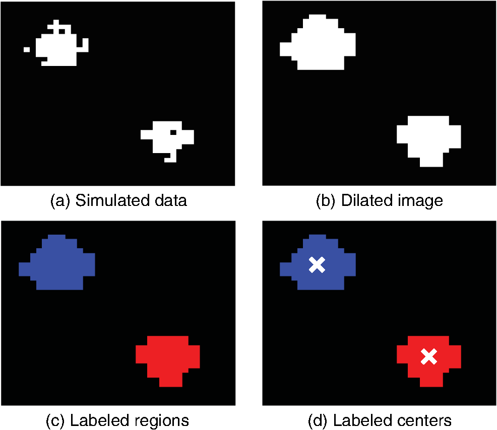 The estimate of the microsphere location was improved and the width of the fluorescence was determined by performing a Gaussian fit on the image. Two-dimensional (2-D) Gaussian images were generated based on Eq. (1) for each value of between 0.1 and 30 in steps of 0.1 The fitting procedure searched a space five pixels on each side of the estimated center value. At each location, the cross correlation was calculated between the measured image and each of the 300 different Gaussian images. An example of the result of these correlations is shown in Fig. 4(a). The correlations and Gaussian parameter , called the width of the fluorescence, were recorded for the best fit at each location. Then, the best correlation across all of the locations was determined as shown in Fig. 4(b). The accurate center location and width of the fluorescence signal were recorded for each microsphere. Fig. 4An improved estimate of sphere location and fluorescence width is determined by finding the best Gaussian fit. (a) For each location, the best fit versus Gaussian width is determined. (b) The best fit at each location is compared to find the best location and width.  Locating microspheres in shadow images were slightly more complex than locating the microspheres in fluorescence images, because all the microspheres in the sample appeared in the shadow image while only those microspheres closest to the imager appeared in the fluorescence image. The larger number of microspheres made it much more likely that two microspheres would appear close to each other. A method was developed for identifying cases where multiple microspheres could lead to incorrect location determination. First, a candidate microsphere location was determined. A window was defined covering 15 pixels in each direction of the microsphere location determined by fluorescence imaging. Then, a test described here was performed to determine if the widow contained only one microsphere as in Fig. 5(a) or multiple microspheres as in Fig. 5(b). A potential center was determined by finding the point with the best correlation to a block. This location is marked by an “” in Fig. 5(c). The single microsphere and multiple microsphere cases were distinguished by first calculating a threshold half way between the minimum and maximum values in the window. Then, the pixels within a box around the identified microsphere were set to zero. If less than five of the remaining pixels were above the threshold, as shown in Fig. 5(d), the location was considered valid. If more than five of the remaining pixels were above the threshold, then the window likely contained more than one microsphere and the location was considered invalid. Fig. 5Shadow images are processed to distinguish between a single microsphere (a) and multiple microspheres (b). For each single microsphere, the center is identified as shown in (c) by finding the best fit to a block. The validity of this fit is then checked by counting the number of dark pixels outside a grid surrounding the center (d).  If the microsphere had valid locations in all five images, the height of the microsphere, , was then calculated using Eq. (3) based on the similar triangles shown in Fig. 1(b): where is the height of the LED and is the displacement of the shadow.Four heights are calculated for each microsphere based on the five shadow images created. The values of these heights are then averaged to determine the height of the microsphere. 2.7.LFI of Flowing SamplesLFI was performed on two types of flowing samples: fluorescent microspheres and cells stained with quantum dots. About 1 μl of the same microspheres used for the calibration was mixed with 500 μl of DI water for this experiment. The cell sample was prepared using RAW 264.7 cells from American type culture collection, Manassas, Virginia and quantum dots from Invitrogen, Grand Island, New York (Q25011MP). The cells were grown on a fibronectin treated glass slide placed inside a humid chamber. The cells were left in the incubator until they covered 80% of the base of the slide. The protocol recommended by Invitrogen was followed to stain the cells except incubation time of cells with the staining solution was increased to 3 h to improve the absorption of quantum dots. The stained cells were then rinsed with fresh media and trypsinized to detach the cells. The detached cells were mixed with the media and loaded in a syringe for the experiment. A simple microfluidic device was fabricated directly on the CMOS imager. First, a design was developed in Autocad. Then, the design was cut out of double-sided tape (Adhesive Research, ARC are 92712, Glen Rock, Pennsylvania) using a laser cutter (Epilog 10000). A PDMS slab was made by mixing the base with the curing agent at a ratio (Sylgard 184). The mixture was poured in a cell culture dish and placed on the hot plate for a few minutes to remove bubbles and left at room temperature over night to cure. A small cube was cut after the PDMS had hardened and ports were punched using a 22 gauge blunt needle. One side of the tape was stuck to the PDMS aligned with the ports and the other side was stuck to the imager. Once the imager set up was ready, PTFE tubing of size 30 from Cole-Parmer, Vernon Hills, Illinois (Part No. EW-06417-11) was inserted into the ports. The input port was attached to a syringe (Easy touch insulin syringe U-100) loaded with the sample. The output port fed a microcentrifuge tube. During imaging, the sample from the insulin syringe was injected into the chamber by a syringe pump (New Era Pump Systems, Inc. NE-1002×, Framingdale, New York) at the rate of . 3.ResultsThe results of this project are divided into simulation results, fluorescence imaging results, shadow imaging results, calibration results between fluorescence and shadow imaging, and results from flowing samples. 3.1.SimulationLFI was simulated for unit spheres at different heights above the imaging sensor as described in Sec. 2. Each simulation produced a 2-D matrix with each value representing the intensity measured by a single pixel of an imaging sensor. The intensities are plotted for a single horizontal line passing through the center of the microsphere image in Fig. 6 to allow for the comparison between different sphere-sensor separations. Fig. 6Lensless fluorescence imaging simulations produced two-dimensional images of microspheres. A single row through the center of each image is presented in this figure to make it possible to compare different sphere-sensor separations. (a) A plot of intensity versus radial distance emphasizes the declining peak with increasing separation. (b) Plotting the same data normalized for the same peak emphasizes the increasing width for increasing separation.  Figure 6(a) is a plot of the fluorescence intensity for four different sphere-sensor separations. As the separation increases, the peak intensity decreases. Beyond four or five times the sphere’s radius, the peak becomes indistinguishable from the background. For typical cells with a radius of 5 to 10 μm, this distance is 25 to 50 μm. Figure 6(b) is a plot of the same curves as Fig. 6(a) but with all the curves normalized to the same maximum value. This format emphasizes the change in shape of the fluorescence curves with the separation. Each of these curves is approximately Gaussian in shape with spheres with greater separation leading to wider curves. 3.2.Lensless Fluorescence ImagingLFI was performed on 226 microspheres in nine samples. Figure 7 shows the basic stages of image processing that were applied to each sample. The same techniques that were applied to simulated data in Fig. 3 were applied here to real data. Figure 8 summarizes the results for four typical microspheres. For each microsphere, the captured image is shown on the left and the plot on the right shows a cross-section view of the captured data and of the Gaussian fit. Moving from Figs. 8(a)–8(d), the intensity decreases and fluorescence width increases. Gaussian curves fit the data well until the broadest peak where noise plays a larger role. The curve fit in Fig. 8(d) highlights the fact that the Gaussian fits were performed on the 2-D data so they may not be the best fit for the one-dimensional data plotted in the figure. Fig. 7The lensless fluorescence image from one to nine samples used in this work shows a large number of fluorescent spheres. (a) The raw data are quite faint with varying intensities. (b) Thresholding makes it easier to identify each sphere. (c) The image is dilated to ensure that each sphere is represented by a single region. (d) The numbering of the regions is denoted by different colors for each region.  Fig. 8Data for individual fluorescence microspheres shows a good match to the Gaussian model. Four fluorescence blobs are shown that span the width of measured images from very narrow (a) to very wide (d). Both the two-dimensional and one-dimensional intensity plot are shown for each microsphere. (a) Very narrow microsphere, (b) narrow microsphere, (c) wide microsphere, and (d) very wide microsphere. 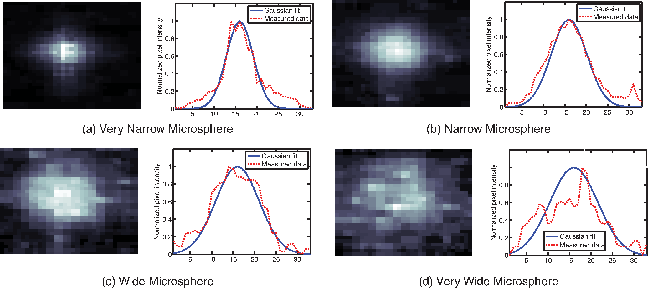 3.3.Shadow ImagingFigure 9 shows that the microsphere shadows are clearly visible when the sample is illuminated from above. The images in Figs. 9(a)–9(e) are the same subsection of shadow images taken from five different illumination angles from the right to the left with Fig. 9(c) taken with illumination from directly above. The four spheres that appear in the five images are labeled in Fig. 9(f). Their paths are tracked across the five images in Fig. 9(g). The greater movement of the microspheres denoted by a star and a square imply that they are higher than the microspheres denoted by a circle and a diamond. Fig. 9The same subset of five shadow images taken of a single sample are shown in (a)–(e). The four spheres labeled in (f) are found in all five shadow images. The movement of each of these four spheres across the five images is shown in (g) to demonstrate the difference in how much different spheres move based on their distance from the sensor.  Of the 226 spheres identified by LFI, only 54 made it through the filtering process described in Sec. 2 to ensure that accurate shadow locations could be calculated for all five images. Their heights are presented as a histogram in Fig. 10. There are a large number of microspheres at 5 μm because these microspheres are resting on the surface of the imager chip approximately 5 μm above the actual sensor elements. No microspheres above 35 μm were recorded because they could not be identified in the lensless fluorescence image. 3.4.3-D Fluorescence Shadow CorrelationThe correlation between 3-D fluorescence images and microsphere heights was determined by plotting the fluorescence width versus the sphere height as shown in Fig. 11. The data is labeled with the run number in which each microsphere was measured to show the repeatability of this method. A line of best fit for the data is described by the equation Fig. 11The relationship between fluorescence diameter and sample separation is linear as shown by this data collected over nine runs and plotted with a best fit line.  Over the range of sphere heights from 5 to 35 μm, the maximum error between the best-fit line and the actual measurement was 7 μm and the standard deviation of the error was 2.6 μm. 3.5.Lensless Fluorescence Imaging of Flowing SamplesCells could not survive the procedure used to suspend microspheres in agarose, so LFI of cells was performed with the cells in liquid suspension. In the first experiment, detached cells stained with quantum dots were mixed with fresh media and placed on the imager and allowed to evaporate. The sample was excited with a UV source and images were captured as the water evaporated. As shown in Fig. 12, despite the more complicated geometry of the cell compared to microspheres, the lensless fluorescence image is still well modeled by a Gaussian curve. Fig. 12Data from individual cells. (a) Cell with high sample-sensor separation. (b) Cell with relatively low sample-sensor separation.  To demonstrate that the technique works with a flowing sample, the imager with the microfluidic device was employed. The sample was pumped into the microfluidic channel and excited with a UV source. A video of the sample flowing through the chambers was captured. Figure 13 contains frames from the video demonstrating movement of microspheres [Figs. 13(a)–13(c)] and cells [Figs. 13(d)–13(f)]. 4.DiscussionFluorescence detection is an attractive technology for integration in lab-on-a-chip systems because it offers high selectivity and sensitivity, but its use has been limited due to the high cost of existing techniques.21 LFI is well suited for integration because it only uses two components, an unfocused light source and an integrated circuit. In this work, the light source was a low-pressure mercury bulb, but in future versions more compact light emitting diodes will likely be used. In addition to performing imaging, the integrated circuit can perform logical control operations, image processing, and communication. This added complexity is especially useful for digital microfluidic devices.22 The biggest challenge to LFI has been the need to tightly control the spacing between the sample and the sensor. In practice, this has limited the technique to applications where the sample is only measured in a thin layer directly on top of the sensor either due to the use of total internal reflection for excitation16 or because the labeled cells are only found at the surface.17,18 The work presented here demonstrates both the tradeoff between separation and LFI performance and a method for measuring separation based on the measured fluorescence image. The data presented in this paper can be used to determine the height of microfluidic channels for LFI in applications that only require fluorescent cell counting. For applications that require 3-D cell tracking, the image processing techniques presented here could be used. As the results show, the functionality of this device can be extended to implement a flow cytometer without increasing the complexity of the imaging system. Delivering these results by employing only an imager and a UV source without the use of any optics makes the device robust, low cost, and easy to use in resource-limited areas. 5.ConclusionThis work has shown that the challenge of tightly controlling the sample-sensor separation for LFI can be relaxed by performing image processing to calculate the height of fluorescently labeled cells. Initial evidence was presented in the form of simulations from first principles. Based on the results of those simulations, an experiment was designed based on the fluorescently labeled spheres. A calibration method by fixing these spheres at precise locations just microns above the imager surface was developed. The height of each sphere was then calculated using a simple trigonometric technique based on shadow imaging. Then LFI was performed on the sample. An image processing technique was developed for estimating the height of the sphere based on only the fluorescence measurement. Finally, LFI was demonstrated in flowing cells in a microfluidic network. AppendicesAppendix:Derivation of Point Illumination PatternA closed form solution for the illumination from a point source can be calculated by considering a point light source at a distance above an infinite plane. The illumination pattern will be axially symmetric about a line perpendicular to the plane going to the point light source. A unit sphere is placed around the point light source. Since the light source is omnidirectional, the light flux will have a constant density throughout the unit sphere. The illumination pattern on the plane can be determined by constructing a right triangle where the hypotenuse is the line between the point in the plane and the light source, one leg is in the plane, and the other leg is perpendicular to the plane. Rotating this right triangle around the symmetry line creates a cone with a disk on the plane. The total illumination within that disk is proportional to the surface area of the unit sphere enclosed by the cone. This area can be calculated using spherical coordinates centered on the point light source The illumination falling on the outside ring of the disk can then be calculated by taking the ratio of the derivatives of growth of the area of the sphere and the area of the disk AcknowledgmentsThis work was supported by the Dev and Linda Gupta Endowment and NSF Grant No. 1128558. ReferencesJ. WolcottA. SchwartzC. Goodman,
“Laboratory medicine: a national status report,”
Prep. Centers Dis. Control Prev.,
(2008). Google Scholar
R. J. Buesa,
“Current status of cytology laboratories in anatomic pathology departments,”
Ann. Diagn. Pathol., 14
(5), 347
–354
(2010). http://dx.doi.org/10.1016/j.anndiagpath.2010.07.005 ANDPFM 1092-9134. Google Scholar
I. BalachandranM. Friedlander,
“Cytology workforce study a report of current practices and trends in New York State,”
Am. J. Clin. Pathol., 136
(1), 108
–118
(2011). http://dx.doi.org/10.1309/AJCPUDFRALJY32XM AJCPAI 0002-9173 Google Scholar
J. L. WeaverM. Stetler-Stevenson,
“Flow cytometry in the biomedical arena,”
Medical Biomethods Handbook, 531
–553 Springer-Verlag, New York
(2005). Google Scholar
M. Alunni-FabbroniM. T. Sandri,
“Circulating tumour cells in clinical practice: methods of detection and possible characterization,”
Methods San Diego Calif., 50 289
–297
(2010). Google Scholar
D. A. Ateyaet al.,
“The good, the bad, and the tiny: a review of microflow cytometry,”
Anal. Bioanal. Chem., 391
(5), 1485
–1498
(2008). http://dx.doi.org/10.1007/s00216-007-1827-5 ABCNBP 1618-2642 Google Scholar
S. C. Linet al.,
“Channel layer, single sheath-flow inlet microfluidic flow cytometer with three-dimensional hydrodynamic focusing,”
Lab Chip, 12
(17), 3135
–3141
(2012). LCAHAM 1473-0197 Google Scholar
S. W. Kettlitzet al.,
“Planar microfluidic chip employing a light emitting diode and a PIN-photodiode for portable flow cytometers,”
Lab Chip, 12 197
–203
(2011). http://dx.doi.org/10.1039/c1lc20672a LCAHAM 1473-0197 Google Scholar
Y. J. FanH. J. SheenP. Y. Chiou,
“High throughput and parallel flow cytometer with solid immersion microball lens array,”
in 2012 IEEE 25th Int. Conf. Micro Electro Mech. Syst. Mems,
1041
–1044
(2012). Google Scholar
A. OzcanU. Demirci,
“Ultra wide-field lens-free monitoring of cells on-chip,”
Lab Chip, 8
(1), 98
–106
(2007). http://dx.doi.org/10.1039/b713695a LCAHAM 1473-0197 Google Scholar
O. Mudanyaliet al.,
“Lensless on-chip imaging of cells provides a new tool for high-throughput cell-biology and medical diagnostics,”
J. Visualized Exp., 34 e1650
(2009). http://dx.doi.org/10.3791/1650 JVEOA4 1940-087X. Google Scholar
T. Suet al.,
“Multi-angle lensless digital holography for depth resolved imaging on a chip,”
Opt. Express, 18
(9), 9690
–9711
(2010). http://dx.doi.org/10.1364/OE.18.009690 OPEXFF 1094-4087 Google Scholar
J. Weidlinget al.,
“Lens-free computational imaging of capillary morphogenesis within three-dimensional substrates,”
J. Biomed. Opt., 17
(12), 126018
(2012). http://dx.doi.org/10.1117/1.JBO.17.12.126018 JBOPFO 1083-3668 Google Scholar
T. SuL. XueA. Ozcan,
“High-throughput lensfree 3D tracking of human sperms reveals rare statistics of helical trajectories,”
Proc. Natl. Acad. Sci. U. S. A., 109
(40), 16018
–16022
(2012). http://dx.doi.org/10.1073/pnas.1212506109 PIPSBD 0370-0046 Google Scholar
T. Suet al.,
“Sperm trajectories from chiral ribbons,”
Sci. Rep., 3 1664
(2013). http://dx.doi.org/10.1038/srep01664 SRCEC3 2045-2322. Google Scholar
A. F. Coskunet al.,
“Lensfree fluorescent on-chip imaging of transgenic Caenorhabditis elegans over an ultra-wide field-of-view,”
PLoS One, 6 e15955
(2011). http://dx.doi.org/10.1371/journal.pone.0015955 1932-6203 Google Scholar
E. P. Dupontet al.,
“Fluorescent magnetic bead and cell differentiation/counting using a CMOS SPAD matrix,”
Sens. Actuators B, 174 609
–615
(2012). http://dx.doi.org/10.1016/j.snb.2012.06.049 SABCEB 0925-4005 Google Scholar
W. Liet al.,
“On-chip integrated lensless fluorescence microscopy/spectroscopy module for cell-based sensors,”
Proc. SPIE, 7894 78940Q
(2011). http://dx.doi.org/10.1117/12.875417 PSISDG 0277-786X Google Scholar
A. F. Coskunet al.,
“Lensfree wide-field fluorescent imaging on a chip using compressive decoding of sparse objects,”
Opt. Express, 18
(10), 10510
–10523
(2010). http://dx.doi.org/10.1364/OE.18.010510 OPEXFF 1094-4087 Google Scholar
H. HanM. KrimanM. Boomgarden,
“Wafer level camera technology—from wafer level packaging to wafer level integration,”
in 2010 11th Int. Conf. Electron. Packag. Technol. High Density Packag. (ICEPT-HDP),
121
–124
(2010). Google Scholar
J. WuM. Gu,
“Microfluidic sensing: state of the art fabrication and detection techniques,”
J. Biomed. Opt., 16
(8), 080901
(2011). http://dx.doi.org/10.1117/1.3607430 JBOPFO 1083-3668 Google Scholar
J. Nicholset al.,
“On-chip digital microfluidic architectures for enhanced actuation and sensing,”
J. Biomed. Opt., 17
(16), 067005
(2012). http://dx.doi.org/10.1117/1.JBO.17.6.067005 JBOPFO 1083-3668 Google Scholar
|


