|
|
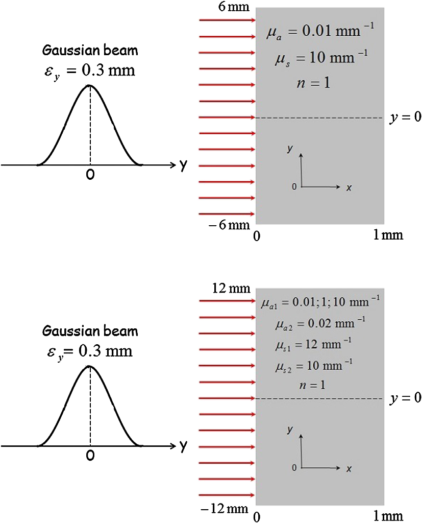
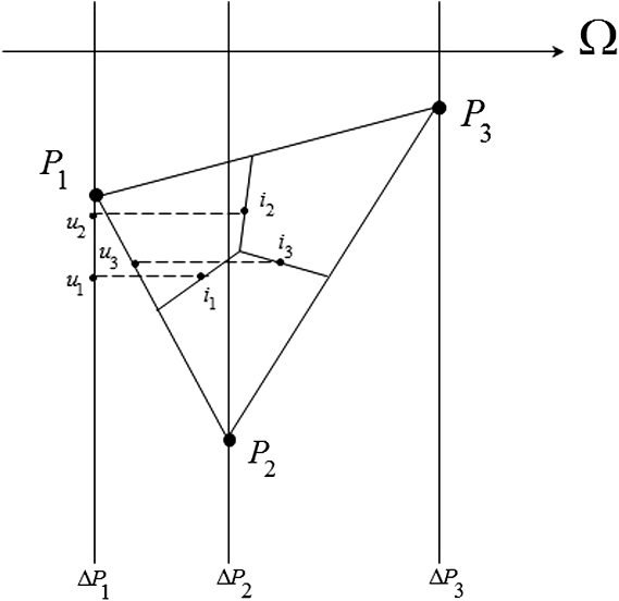
1.IntroductionThe use of visible or near-infrared light provides many possibilities, particularly for applications in biomedical treatment and diagnosis, such as optical tomography, laser surgery, and photodynamic therapy. To develop an efficient tool, it is essential to have high-order accuracy models for predicting light propagation within inhomogeneous, absorbing, and highly forward-scattering media, typical for biological tissues. Modeling of light propagation through biological tissues has traditionally been done with the diffusion approximation (DA)1,2 or the statistical Monte Carlo (MC) method.3–11 The diffusion theory presumes that the scattering is predominate and that the medium is optically diffuse so that the angle-dependent radiant intensity is replaced by an angle-independent photon flux and the radiative transfer equation (RTE) is simplified as a diffusion equation. However, the DA is hardly applicable to heterogeneous biological tissues with nonscattering or low-scattering regions; moreover, experiments2 have shown that it fails to match experimental data when the tissue sample is not optically diffuse. The MC technique was broadly used because of its simple algorithm and flexibility to include real physical conditions. Nethertheless, this method requires a large number of photons to obtain smooth accurate solutions, which is highly time consuming. Alternatively, different (deterministic) numerical methods have been developed to solve the RTE in the spatial domain, for example, the finite difference method,12–15 the finite element method (FEM),16,17 or the finite volume method (FVM).18 By using an angular discretization of the RTE, the cited methods are considered as a discrete ordinates method (DOM).19 It is known that one of the more serious shortcomings of the DOM is false scattering, which is a consequence of spatial discretization errors. Another serious drawback of the method is the so-called ray effect, which is a consequence of angular discretization (see, for example, chapter 16 in Ref. 19). In our earlier work, a modified FVM (MFVM) for solving the two-dimensional (2-D) RTE has been developed.20 Recently, two authors of the present paper succeeded in deriving exact analytical solutions to the RTE for a variety of different geometries.21–23 It has to be emphasized that these exact analytical solutions are very useful for validation of the numerical methods. This paper presents a comparison between three different solutions of the RTE based on the MFVM,20 the analytical approach,21,22 and the MC technique6 for predicting light propagation within absorbing and highly forward-scattering media, subjected to a collimated light beam. Few works can be found in the literature on the same topic.24–28 In Ref. 24, calculations based on the DA, the DOM for solving the RTE in the time domain, and the MC technique were conducted and compared for predicting light transport in multidimensional biological tissues. In that case, the DA were solved with the FEM using a commercial package FEMLAB. Comparisons among the three methods were performed over a broad range of parameters, such as the scattering and absorption coefficients, the heterogeneity of the tissues, the CPU time, etc. It was concluded that the DOM was found to closely match the MC simulation. Da Silva et al.25 compared the auxiliary function method (giving an exact solution) and the DOM for a heterogeneous absorbing and scattering (one-dimensional) slab composed of a single flat layer or a multilayer in the steady-state domain. The comparison was applied to two different media presenting two typical and extreme scattering behaviors: Rayleigh and Mie scattering with smooth or very anisotropic phase functions, respectively. A good agreement between the two methods was observed in both cases. Mishra et al.26 studied numerically a square short-pulse laser having pulse-width of the order of a femtosecond on transmittance and reflectance signals in case of an absorbing and scattering planar layer. A comparison of the performance of the three numerical methods for solving the RTE, namely, the discrete transfer method, the DOM, and the FVM, was performed. Effects of the optical properties (extinction coefficient, scattering albedo, anisotropy factor) and the laser properties, such as the pulse-width and the angle of incidence, on the transmittance and the reflectance signals were compared. In all the cases, results of the three methods were found to compare very well with each other. Computationally, the DOM was found to be the most efficient. In Ref. 27, a comparison of light transport models in view of optical tomography applications was performed. These models were based on two FEMs associated with the DOM (for solving the 2-D RTE in the steady-state domain), namely, the least square and the discontinuous Galerkin finite element (DGFE) formulations. The comparison of both methods using the and the angular quadratures shows that the DGFE gives more accurate solutions for problems with strong discontinuities, but may exhibit some oscillations due to the Galerkin procedure. A test on a collimated irradiation showed that both methods give the same accuracy due to the separation of the radiance into collimated and diffuse components, which removes the discontinuities in the implementation of the boundary conditions. Recently, the RTE in the time domain was solved for an axisymmetric cylindrical medium using both the DOM and the FVM.28 Steady and transient flux profiles were determined for absorbing and scattering media. Results for each solution method were compared and shown for various grid numbers, scattering albedos, and optical thicknesses. A comparison of CPU time and memory usage among the methods was presented. It was found that the FVM uses more memory and has a longer convergence time than the DOM for all cases due to the difference in angular treatment. The remainder of this paper is organized as follows. Section 2 deals with the problem statement for 2-D geometries and gives details of the MFVM. In our previous publication,20 only homogeneous biological media have been considered and the boundaries were assumed to be transparent. Also, some extensions of the numerical method, regarding the space-varying optical properties and the interface between two media (refractive index mismatch with Fresnel reflection at the interface), have been developed for the present work. Moreover, more complex collimated light beams and a new time semi-discretization of the RTE are employed here. The third section analyzes and discusses the comparison results among the different methods cited above. The last section reports our conclusions and suggests further developments for this work. 2.Numerical Treatment of the Radiative Transfer Equation2.1.Modified Finite Volume Method2.1.1.Problem statementA 2-D absorbing and highly forward-scattering medium, such as biological tissue exposed to arbitrary collimated external radiation, is analyzed. Except for the refractive index, which is constant, the medium has nonuniform optical properties to model, in the present study, a homogeneous or a two-layered medium and, in the future, the complex heterogeneities inside biological tissues. The external radiation that penetrates from the outside into the participating medium is brought by a perpendicular collimated light beam. One part of it propagates in the medium without being deviated, while the other part is scattered in all directions of space. Then, it is convenient to split the radiance into two components denoted as , where is the collimated radiance (), is the spatial position (mm), is the direction vector, and is the time (ps), and , which are, respectively, the collimated and diffuse components of light.19 The intensity () of the collimated light beam is , given at any location point on the bounding surface that is illuminated. Then, the collimated radiance is governed by Bouguer-Beer-Lambert attenuation law. where is the refractive index, is the speed of light in vacuum (0.299793 ), is the attenuation coefficient (), is the Dirac-delta function, is the direction of the collimated light beam, and . The diffuse radiance is solution of the RTE with an additional radiation source term () () due to the scattered part of the collimated light beam.19,20 where is the scattering coefficient () and is the scattering phase function (). The scattering phase function describes the probability that a light beam from one direction, , will be scattered into a certain other direction . The fluence () and the outgoing flux at the (transparent) bounding surface of the medium can be calculated, respectively, as where the contribution of is valid only for . is the local unit surface normal pointing into the medium. It should be noted that the reflectance (respectively transmittance) corresponds to the outgoing flux at the bounding surface (resp. opposite bounding surface) that is illuminated.2.1.2.Discretization of the time, angular, and spatial domainsThe time domain was discretized with a constant step such that , where was the number of iteration. The angular space () was uniformly subdivided into discrete directions, . The computational spatial domain was divided into three-node triangular elements using unstructured (or structured) meshes. As in Ref. 20, a cell-vertex formulation29 was adopted in this work to have a high resolution in space of the RTE. It consists of building control volumes around each node of the mesh and computing the solution at the nodes of the mesh (nodes of triangles). The polygonal control volumes connected to each node were built by joining the centroids of the elements to the midpoints of the corresponding sides (Fig. 1). Control volumes surrounding the nodes at the boundaries of the medium were built as illustrated in Ref. 30. The surface of the control volume related to node was subdivided into surface elements. For a surface element , was the integration point located at the center of the surface element, was its surface area () and, was the local unit outward normal vector. It should be noted that the integration points of panels are defined only from the coordinates of the vertices of triangles of the mesh (Fig. 1). 2.1.3.Full discretization of the RTEFVM applied to the RTE for the spatial domainThe integration of the RTE over a control volume () (Fig. 1) and into a discrete solid angle centered around an discrete direction yields19,20 where is the radiance defined at time and at position traveling in the direction of unit vector [located here in the plane ] where light propagates at the velocity in the medium. is the radiation source term given by Eq. (2). By applying the divergence theorem to the second term of the left member of Eq. (4), it follows thatLet be an approximation of the radiance at time , and at the integration position traveling in the discrete direction. Then, Eq. (5) is approximated by It should be noted that is an integral that depends only on the orientation of surface element for the direction considered. This quantity is calculated in an exact way.30 We assume that (, ) and optical properties (, ), where is the absorption coefficient (), are constant inside a sufficiently small control volume (taking only one value at node ) and inside . The full discretization of the steady-state Eq. (4) yields the following algebraic equation: where and represents the average part of the scattered energy from the control solid angle toward the control solid angle .20Spatial discretization of the transport term of the radianceTo solve Eq. (7), closure relations between the integration-point values and the nodal values of the radiance are required (Fig. 1). The directional nature of radiative transfer needed to be taken into account in order to establish the closure relations. Thus, for a specific direction of propagation of light, only the nodal values located upstream from the integration point had to be considered. In the same way, as presented in Ref. 20, a locally rigorous one-dimensional integration of the RTE along the optical path has to be used. Here, and are assumed to be on the same optical path of direction with located upstream from and . The following approximation can be used, . To compact the equations, the following notations are introduced: From Eqs. (2) and (8), an approximate value of can be deduced. The computation of integrals in Eq. (10) is detailed in Appendix B. Combining Eqs. (9) and (10) in Eq. (6) gives where is the azimuthal angle (rad). The projections and linear interpolations presented in Ref. 30 were expected to improve the closure relations and the accuracy of the results. Also, they were used and generalized in this study to link defined at the point with the nodal values of the radiance (see Appendix A).Full discretization of the RTEThe formula for the fourth-order Runge-Kutta (RK4)31 was used for the time semi-discretization of Eq. (4) combined to discrete Eq. (7). We also tested the formula for the Runge-Kutta-Fehlberg method (RK45), which is known to be more precise than RK4, but the results were similar. An iterative procedure is required to solve equations in the time domain (and also in the steady state). Inspection of these equations shows that they can only be solved for one prescribed discrete direction. To evaluate the sums over in Eqs. (7) and (12), it is necessary to know, as preliminary at time (respectively at iteration in the steady state), the specific radiances and in all discrete directions . In our case, these specific radiances were changed by the same one computed at the previous iteration since the values are known at time (respectively at iteration in the steady state). The convergence criterion was related to a relative difference dealing with the values of the outgoing flux at the bounding surface of the medium. In all results presented further, the iterations have been achieved with a relative difference that does not exceed a prescribed tolerance set to . Moreover, our numerical method is designed to take into account mismatched interfaces as described in Appendix C. The MFVM described above was coded using C language. A particular effort has been done over the optimization of data structures and computations in the sequential code. As all real numbers manipulated in the code are coded in double precision to ensure a high accuracy of the results, a trade-off has been required between memory consumption and computational time in the context of sequential execution on a single computer. However, this constraint may be at least partially relaxed in a context of cluster computing, implying the use of several computers and thus, a larger aggregated memory. Moreover, even in the context of a single computer, there is a great potential of computational time reduction by using the multiple cores present in current computers and/or GPUs. 2.2.Monte Carlo TechniqueThe MC technique simulates the photons’ paths in the considered scattering medium according to the probability functions for the involved physical quantities like the absorption coefficient, the scattering coefficient, and the scattering phase function. During or after the simulation of each photon’s path, the information of the requested quantities, like the location of reflectance, is scored. Upon calculating a large number of photons, these quantities converge to the exact solution of the RTE.21 In this study, the 2-D MC simulations were performed with a modified version22 of a three-dimensional (3-D) code described in detail elsewhere.6 The modification mainly consisted of holding the azimuthal angle fixed at a constant value and using the 2-D Henyey-Greenstein function as scattering function. As in the 3-D code, Fresnel’s formulae were applied at the boundaries of the scattering media. In the time domain, the reflectance was calculated by converting the photons’ path lengths into time via the speed of light in the scattering medium. 2.3.Analytical SolutionThe analytical approach for solving the 2-D RTE is based on an infinite Fourier transform regarding one spatial coordinate as well as on a Fourier series for the angular coordinate.23 The resulting eigenvalue problem is solved via an eigenvalue decomposition of a simple symmetric tridiagonal matrix, which has to be performed once only. The boundary condition is satisfied by using a Marshak-type boundary condition.23 3.Results and DiscussionIn this section, the obtained solutions with the MFVM are validated against the analytical approach and the MC technique. The Henyey-Greenstein phase function has been used to account for the anisotropic nature of scattering by the medium. This function, which depends only on the scalar product between the incident direction and that scattered and the anisotropy factor , is expressed for 2-D media as32 In all the cases presented further, is set to 0.9, which corresponds to highly forward-scattering media, such as biological tissue. The refractive index of the outside medium (air) is equal to 1. In the first three cases, the steady state is considered and the bounding surface of the medium at was illuminated with a perpendicular collimated Gaussian beam having a spatial intensity of with set to 0.3 mm in all simulations. The angular space () was uniformly subdivided into control solid angles to obtain a converged solution of the MFVM in the angular domain. Furthermore, sensitivity studies of the MFVM were carried out on spatial discretization with four different structured spatial meshes composed of () nodes [ according to the axis]. Mesh , ; Mesh , ; Mesh , ; Mesh , . Each spatial mesh was refined according to the axis near the zone of interest corresponding to the section . The calculations were carried out with a computer of 2.56 GHz, 12 GB for the MFVM and with a computer of 2.5 GHz, 4 GB for the MC.3.1.Homogenous Slab (Case 1)The first test case, taken from Ref. 22, deals with a homogenous slab. The boundaries of the medium are assumed to be transparent. The optical properties of the medium [Fig. 2(a)] are typical for biological tissue in the near-infrared spectral range, where the absorption coefficient is particularly low. It should be noted that the medium is optically thick (10.01), and thus the regime of multiple scattering has to be considered [, where is the thickness of the medium (mm), is the scattering mean free path (), and is the absorption mean free path ()]. To correctly take into account the first scattering events in the medium (), the first node of the grid [according to the axis] from the bounding surface of the medium at was located at 0.033 mm for mesh 1, 0.025 mm for mesh 2, and 0.016 mm for meshes 3 and 4. The steady-state spatially resolved reflectance (at ) and transmittance (at ) are shown in Fig. 3(a). Due to the relatively small thickness, the magnitudes for reflectance and transmittance decrease strongly when spatial position increases. It can be seen that the numerical solution given by the MFVM is in good agreement with the exact analytical solution.22 False scattering and ray effect cause mainly the relative differences between the two solutions, and a potential way to reduce it is to use a spatial mesh refinement [as illustrated in Fig. 3(b)] accompanied by a finer angular quadrature. The differences are higher for transmittance. The relative differences for reflectance are (meshes 1 and 2) and 1% (mesh 3), respectively. For transmittance, they are (mesh 1), 3.4% (mesh 2), and 2.4% (mesh 3), respectively. The diffuse fluence inside the medium is depicted in Fig. 4, and we can seen a symmetry plane mm and forward light scattering, which is in agreement with the value of . The diffuse fluence is concentrated in the region between and . These imply that the relative difference for transmittance has peaked regions [Fig. 3(b)] between and . A uniform angular quadrature was used in this work. A potential way to reduce the relative difference for transmittance is to use a nonuniform angular quadrature and to refine it near the zone of the collimated direction. 3.2.Refractive Index Mismatch with Fresnel Reflection at the Interface (Case 2)The medium studied in this section has a refractive index equal to 1.4 and the boundaries of the medium are assumed to be semitransparent (see Appendix C). The other parameters are the same as in case 1. The steady-state spatially resolved reflectance (at ) and transmittance (at ) are depicted in Fig. 5(a). Compared to case 1, the magnitudes for reflectance and transmittance are lower for near to 0. It is due to the reflected light at the boundaries of the medium directed back into the medium. At the same time, it contributes to give higher magnitudes for reflectance and transmittance when increases. The numerical solution given by the MFVM compares well with the MC solution6 taken as the reference solution in this case. Also, the relative differences between the two solutions [Fig. 5(b)] decrease with spatial mesh refinement, and the differences are higher for transmittance. The relative differences for reflectance are almost always (meshes 1, 2, 3) except for , but this is due to the statistical errors of the MC method, which increase with larger values. For transmittance, they are (mesh 1), 3% (mesh 2), and 2.2% (mesh 3), respectively. The number of simulated photons with MC was 3 and the computational time was 112 min for this case. The computational times required by the MFVM were, respectively, 31 min (mesh 1), 80 min (mesh 2), and 131 min (mesh 3). 3.3.Two-Layered Medium (Case 3)A two-layered medium having a relatively thin first layer of thickness 0.1 mm and a second layer of thickness 0.9 mm is studied. The boundaries of the medium are assumed to be transparent. The values of optical properties of the medium are shown in Figs. 2(b) and 6. In Fig. 6, the steady-state spatially resolved reflectance (at ) are presented for three different absorption coefficients of the first layer (, 1, and ). As expected, the reflectance decreases when the absorption coefficient of the first layer increases. The results show a good agreement between the numerical solution given by the MFVM and the MC solution.6 The relative differences between the two solutions are higher for and lie between 0 and 5% [Fig. 6(b)]. For the two other absorption coefficients of the first layer, the relative differences are globally . 3.4.Results in the Time Domain (Case 4)The last test case was chosen to evaluate the performance in the time domain of the numerical scheme of the RTE. The optical properties of the homogeneous medium and the boundaries of the medium are the same as in case 1. The Courant-Friedrich-Levy (CFL) condition needs to be satisfied, namely, , where is the size of the smallest cell of the spatial mesh.13 In other words, since a light beam always travels with a velocity corresponding to the speed of light in the medium, the traveling distance between two consecutive time steps should not exceed the size of the smallest cell. The CFL condition was satisfied in our simulations by setting for mesh 3. As initial condition (), there is no light (or photons) in the medium before light impingement. At subsequent times, the bounding surface of the medium at was illuminated with a perpendicular collimated Gaussian beam in space and in time. where is given by Eq. (14), and where is a constant positive time value. For the simulations presented further, , , and . The curves of time-resolved reflectance (at ) are presented for different spatial positions, namely, (Fig. 7). A close shape of the Gaussian pulse in time [Eq. (16)] is found. The curves of reflectance decrease with the increase of -coordinate due to the light propagation. An agreement between the MFVM-RK4 and MC solutions can be seen in Fig. 7(a). However, the relative differences in the time domain are higher than in the steady state. The relative differences increase with the -coordinate and for long times. They are related to the time discretization error of the RTE but also to the statisical error in the MC simulation.The number of simulated photons with MC was and the computational time was 148 min. The computational time required by the MFVM-RK4 to carry out 7000 iterations (direct solution in the time domain) was approximately five days. 4.ConclusionAn MFVM for predicting light propagation within 2-D absorbing and highly forward-scattering medium subjected to a collimated Gaussian light beam has been presented. The accuracy of the MFVM has been examined by comparing the results with an exact analytical solution of the RTE and the MC technique. Numerical results for the spatially resolved reflectance and transmittance over different situations (refractive index mismatch with Fresnel reflection at the interface, homogeneous and two-layered media) have shown that the MFVM yields accurate results. In the steady state, relative differences of the different solutions were found to decrease with spatial mesh refinement obtaining compared to analytical and MC solutions. In the time domain, the RK4 has been used for the time semi-discretization of the RTE. An agreement between the MFVM-RK4 and MC solutions has been shown, but the relative differences were found to be higher than in the steady state. In our future work, we are interested to implement another technique for the time semi-discretization of the RTE as recently proposed in Ref. 33. The technique is based on solving the RTE in the frequency domain at multiple modulation frequencies. It has been reported by the authors that using the Fourier-series representation of the radiance, the solution can be obtained in the time domain with good accuracy and with significantly fewer computational resources than are needed in the direct solution in the time domain. Moreover, the MFVM presented in this paper will be extended to 3-D geometry for biomedical applications, such as diffuse optical tomography for tumor diagnosis. Several aspects of parallel computing for 2-D/3-D MFVM code will be explored to speed up the computation, such as the multithreaded computation (the use of multiple cores present in the same computer), the potential use of GPUs, and the larger scale of parallelism making use of multiple computers in order to manage larger and more complex problems. Our preliminary studies on the parallel computing of the MFVM over direction (in our simulations, typically 128 discrete directions were used) show that we can expect significant gains in computing speed. AppendicesAppendix A:Projections and Linear InterpolationsTo simplify, a notation was introduced: means point is upstream from point . A specific direction of light and a reference triangle denoted by with are considered (Fig. 8). are the planes orthogonal to the direction and that pass, respectively, by . The integration points are related to the triangle. Except in particular cases such as boundaries of the medium (see Ref. 30 for the details), points and are always built in the same way. The integration points are projected on lines perpendicular to the direction and located upstream from points and , the line in the case of points and (Fig. 8). The point is the intersection point, located upstream from , between the direction and the first side met of an element of . Thus, only two cases can arise: is on the line or it is on the line . In our case, radiances at points are approximated by linear interpolation with the values of the closest upstream nodes. The reader is referred to Refs. 20 and 30 for details about this method. Appendix B:Evaluation of the Integral Terms Along an Optical PathLet and be two triangles that have and , respectively, as vertices (Fig. 9). The spatial discretization of the transport term of the radiance leads to the computation of the integrals given below. where is the curvilinear abscissa along the optical path between the points and in the specific direction of light (Fig. 9). The computation of , , and requires knowledge of functions and along this optical path, but these functions are only known at nodes of the mesh . Let , , and . Then, is approximated by a linear interpolation using the value of at the three vertices of . In the same way, is approximated using the value of at the three vertices of . Let be the point (belonging to ) of coordinates . Similarly, let be the point of coordinates . Then, belongs to the plane if and only ifThen, an approximate value of can be deduced: , with The point (which belongs to ) is approximated in the same way. By using the previous relations and the numerical integration with the midpoint rule, it follows that Changing by in Eq. (17) and using the approximation , it follows that Appendix C:Refractive Index MismatchThe real part of the complex refractive index of the medium and the outside medium (air) are denoted as and , respectively. Partial reflection of light at the medium–air interface is caused by the refractive index mismatch of both media, and the fraction of reflected light is given by the directional reflection coefficient . For a semitransparent interface illuminated by an external light source , the partly reflecting boundary specifies the radiance as the sum of two contributions.19,34 where is the specular reflection of . The angle satisfies , where is the angle between two directions and is the local unit outward normal vector. The directional reflection is given by Snell-Descartes laws. Considering that ( being the real and imaginary parts of the complex refractive index, respectively) with , and is the relative refractive index between the two media. The critical angle satisfies Snell’s law: . In our application, , , and . In the particular case of the collimated direction (), . The outgoing flux at the semitransparent bounding surface of the medium isTo solve the RTE with the boundary condition [Eq. (20)], it is necessary to know, as preliminary at time (respectively, at iteration in the steady state), the radiance in the specific direction. In our case, this radiance was changed by the same one computed at the previous iteration since the values are known at time (respectively, at iteration in the steady state). The convergence criterion was related to a relative difference dealing with the values of the outgoing flux at the bounding surface of the medium. In all results presented further, the iterations have been achieved with a relative difference that does not exceed a prescribed tolerance set to . ReferencesA. Ishimaru, Wave Propagation and Scattering in Random Media, Academic Press, New York
(1987). Google Scholar
K. M. YooF. LiuR. R. Alfano,
“When does the diffusion approximation fail to describe photon transport in random media,”
Phys. Rev. Lett., 64 2647
–2650
(1990). http://dx.doi.org/10.1103/PhysRevLett.64.2647 PRLTAO 0031-9007 Google Scholar
B. C. WilsonG. Adam,
“A Monte Carlo model for the absorption and flux distributions of light tissue,”
Med. Phys., 10 824
–830
(1983). http://dx.doi.org/10.1118/1.595361 MPHYA6 0094-2405 Google Scholar
S. T. Flocket al.,
“Monte-Carlo modeling of light propagation in highly scattering tissues. I. Prediction and comparison with diffusion theory,”
IEEE Trans. Biomed. Eng., 36 1162
–1168
(1989). http://dx.doi.org/10.1109/TBME.1989.1173624 IEBEAX 0018-9294 Google Scholar
S. L. Jacques,
“Time resolved propagation of ultrashort laser pulses within turbid tissues,”
Appl. Opt., 28
(12), 2223
–2229
(1989). http://dx.doi.org/10.1364/AO.28.002223 APOPAI 0003-6935 Google Scholar
A. Kienle,
“Lichtausbreitung in biologischem Gewebe,”
University of Ulm,
(1995). Google Scholar
M. Q. BrewsterY. Yamada,
“Optical properties of thick, turbid media from picosecond time-resolved light scattering measurements,”
Int. J. Heat Mass Transf., 38 2569
–2581
(1995). http://dx.doi.org/10.1016/0017-9310(95)00013-Y IJHMAK 0017-9310 Google Scholar
Z. GuoS. KumarK. C. San,
“Multi-dimensional Monte Carlo simulation of short pulse laser radiation transport in scattering media,”
J. Thermophys. Heat Transfer, 14 504
–511
(2000). http://dx.doi.org/10.2514/2.6573 JTHTEO 0887-8722 Google Scholar
Z. Guoet al.,
“Monte Carlo simulation and experiments of pulsed radiative transfer,”
JQSRT, 73 159
–168
(2002). http://dx.doi.org/10.1016/S0022-4073(01)00203-5 JQSRAE 0022-4073 Google Scholar
D. A. Boaset al.,
“Three dimensional Monte Carlo code for photon migration through complex heterogeneous media including the adult human head,”
Opt. Express, 10 159
–170
(2002). http://dx.doi.org/10.1364/OE.10.000159 OPEXFF 1094-4087 Google Scholar
C. ZhuQ. Liu,
“Review of Monte Carlo modeling of light transport in tissues,”
J. Biomed. Opt., 18
(5), 050902
(2013). http://dx.doi.org/10.1117/1.JBO.18.5.050902 JBOPFO 1083-3668 Google Scholar
O. Dorn,
“A transport-backtransport method for optical tomography,”
Inverse Probl., 14
(5), 1107
(1998). http://dx.doi.org/10.1088/0266-5611/14/5/003 INPEEY 0266-5611 Google Scholar
Z. GuoS. Kumar,
“Discrete-ordinates solution of short-pulsed laser transport in two-dimensional turbid media,”
Appl. Opt., 40
(19), 3156
–3163
(2001). http://dx.doi.org/10.1364/AO.40.003156 APOPAI 0003-6935 Google Scholar
M. SakamiK. MitraP.-f. Hsu,
“Analysis of light pulse transport through two-dimensional scattering and absorbing media,”
JQSRT, 73 169
–179
(2002). http://dx.doi.org/10.1016/S0022-4073(01)00216-3 JQSRAE 0022-4073 Google Scholar
J. BoulangerA. Charette,
“Reconstruction optical spectroscopy using transient radiative transfer equation and pulsed laser: a numerical study,”
JQSRT, 93 325
–336
(2005). http://dx.doi.org/10.1016/j.jqsrt.2004.08.028 JQSRAE 0022-4073 Google Scholar
T. TarvainenM. VaukhonenS. R. Arridge,
“Gauss-Newton reconstruction method for optical tomography using the finite element solution of the radiative transfer equation,”
JQSRT, 109 2767
–2778
(2008). http://dx.doi.org/10.1016/j.jqsrt.2008.08.006 JQSRAE 0022-4073 Google Scholar
P. S. Mohanet al.,
“Variable order spherical harmonic expansions scheme for the radiative transport equation using finite elements,”
J. Comput. Phys., 230 7364
–7383
(2011). http://dx.doi.org/10.1016/j.jcp.2011.06.004 JCTPAH 0021-9991 Google Scholar
K. RenG. BalA. H. Hielscher,
“Frequency domain optical tomography based on the equation of radiative transfer,”
SIAM J. Sci. Comput., 28
(4), 1463
–1489
(2006). http://dx.doi.org/10.1137/040619193 SJOCE3 1064-8275 Google Scholar
M. Modest, Radiative Heat Transfer, 2nd Ed.Academic Press, San Diego
(2003). Google Scholar
F. AsllanajS. Fumeron,
“Applying a new computational method for biological tissue optics based on the time-dependent two-dimensional radiative transfer equation,”
J. Biomed. Opt., 17
(7), 075007
(2012). http://dx.doi.org/10.1117/1.JBO.17.7.075007 JBOPFO 1083-3668 Google Scholar
A. LiemertA. Kienle,
“Exact and efficient solution of the radiative transport equation for the semi-infinite medium,”
Sci. Rep., 3 2018
(2013). http://dx.doi.org/10.1038/srep02018 2045-2322SRCEC3 2045-2322 Google Scholar
A. LiemertA. Kienle,
“Analytical approach for solving the radiative transfer equation in two-dimensional layered media,”
JQSRT, 113
(7), 559
–564
(2012). http://dx.doi.org/10.1016/j.jqsrt.2012.01.013 JQSRAE 0022-4073 Google Scholar
A. LiemertA. Kienle,
“Green’s functions for the two-dimensional radiative transfer equation in bounded media,”
J. Phys. A: Math. Theor., 45
(17), 175201
(2012). http://dx.doi.org/10.1088/1751-8113/45/17/175201 1751-8113 Google Scholar
C. Kosarajuet al.,
“Comparison between different forward models for light transport in tissues,”
in Proc. of Asian Symp. on Biomedical Optics and Photomedicine,
108
–109
(2002). Google Scholar
A. Da Silvaet al.,
“Comparison of the auxiliary function method and the discrete-ordinate method for solving the radiative transfer equation for light scattering,”
JOSA, 20
(12), 2321
–2329
(2003). http://dx.doi.org/10.1364/JOSAA.20.002321 JOSAAH 0030-3941 Google Scholar
S. C. Mishraet al.,
“Development and comparison of the DTM, the DOM and the FVM formulations for the short-pulse laser transport through a participating medium,”
Int. J. Heat Mass Transf., 49 1820
–1832
(2006). http://dx.doi.org/10.1016/j.ijheatmasstransfer.2005.10.043 IJHMAK 0017-9310 Google Scholar
O. BalimaA. CharetteD. Marceau,
“Comparison of light transport models based on finite element and the discrete ordinates methods in view of optical tomography applications,”
J. Comput. Appl. Math., 234
(7), 2259
–2271
(2010). http://dx.doi.org/10.1016/j.cam.2009.08.083 JCAMDI 0377-0427 Google Scholar
B. HunterZ. Guo,
“Comparison of discrete-ordinates method and finite volume method for steady-state and ultrafast radiative transfer analysis in cylindrical coordinates,”
Numer. Heat Transf. B, 59
(5), 339
–359
(2011). http://dx.doi.org/10.1080/10407790.2011.572719 NHBFEE 1040-7790 Google Scholar
G. Yuet al.,
“Comparative studies on accuracy and convergence rate between the cell-centered scheme and the cell-vertex scheme for triangular grids,”
IJHMT, 55 8051
–8060
(2012). http://dx.doi.org/10.1016/j.ijheatmasstransfer.2012.08.042 IJHMAK 0017-9310 Google Scholar
F. AsllanajV. FeldheimP. Lybaert,
“Solution of radiative heat transfer in 2D geometries by a modified finite-volume method based on a cell-vertex scheme using unstructured triangular meshes,”
Numer. Heat Transf. B, 51
(2), 97
–119
(2007). http://dx.doi.org/10.1080/10407790600762805 NHBFEE 1040-7790 Google Scholar
E. HairerG. Wanner, Solving Ordinary Differential Equations II. Stiff and Differential-Algebraic Problems, Springer Series in Computational Mathematics, New York
(1991). Google Scholar
J. Heinoet al.,
“Anisotropic effects in highly scattering media,”
Phys. Rev. E, 68 031908
(2003). http://dx.doi.org/10.1103/PhysRevE.68.031908 PLEEE8 1063-651X Google Scholar
A. PulkkinenT. Tarvainen,
“Truncated Fourier-series approximation of the time-domain radiative transfer equation using finite elements,”
J. Opt. Soc. Am. A Opt. Image Sci. Vis., 30
(3), 470
–478
(2013). http://dx.doi.org/10.1364/JOSAA.30.000470 JOAOD6 0740-3232 Google Scholar
A. D. Klose,
“Radiative transfer of luminescence light in biological tissue,”
in Light Scattering Reviews 4,
293
–345
(2009). Google Scholar
|