2.1.

Finite Difference Time Domain Method

The numerical technique that has been used in this work to solve Maxwell’s equations is the FDTD method, which offers a solution for complex scattering geometries.¹³ The developed code was implemented using MATLAB. The injection of the incident beam is achieved using the total-field/scattered-field method (TF/SF). In this method, the FDTD grid is divided into two regions (see Fig. 1). The inner region is the total-field region, where the scatterers are located and the fields resulting from the interaction between the scatterers and the incident fields are calculated. In the second region, the scattered-field region, which surrounds the total-field region, only the scattered fields exist. Only the value of the incident field at the boundary between the two regions is needed for the introduction of the incident field into the FDTD grid. This is advantageous since we do not need to store the incident field everywhere in the grid. Thus, it is necessary to calculate an incident field, which is propagating in an arbitrary direction, and then it is possible to store it so that it can be used to update the boundary between the two regions.¹³ This is done by propagating and saving a one-dimensional (1-D) wave, and then projecting it on the two-dimensional (2-D) grid. Special care needs be taken to minimize any numerical dispersion that occurs due to the 1-D wave not coinciding with the simulation rectangular grid for large oblique angles.¹³

Fig. 1

The implementation of the angular spectrum of plane waves method in the finite difference time domain (FDTD) method. The plane wave propagates in the $x$-direction and passes through a lens where a focused beam is formed at position $(x_0,y_0)$. The FDTD grid is divided into a total field region that contains both the incident and the scattered fields and a scattered field region, which contains only the scattered fields. The incoming wave enters the FDTD grid at the interface between total and scattered field. $y_m$ represents the maximum distance from the focus of the beam to the lateral boundary of the total field and scattered field regions.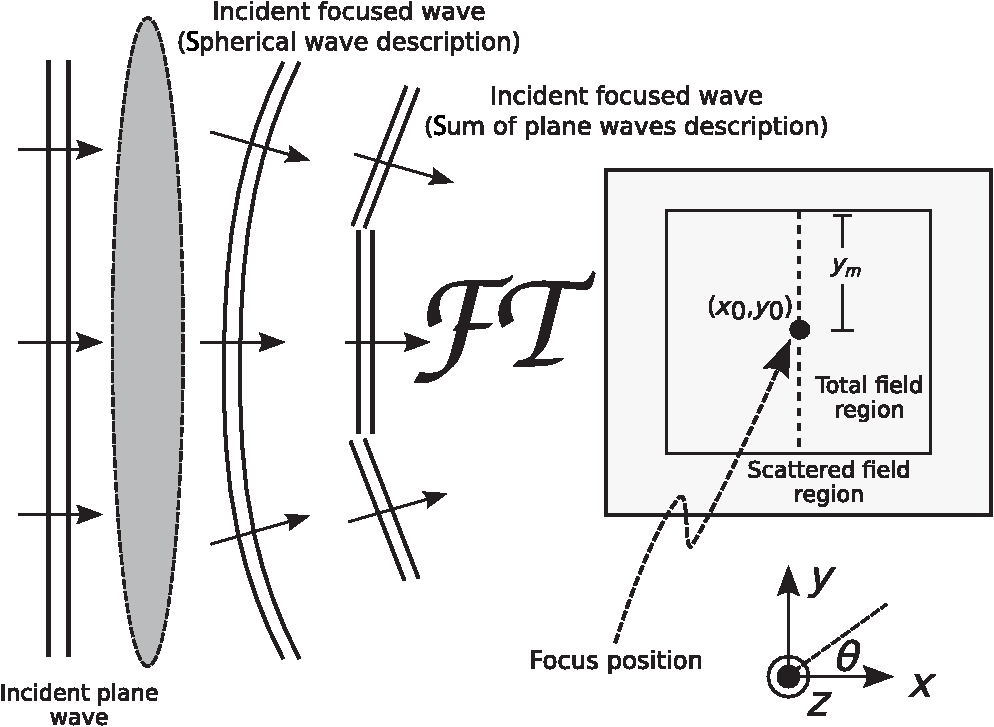

The TF/SF method gives the ability to calculate the scattered near fields and to transform these fields to the far-field solution using appropriate near to far-field transformations. The mathematical description of such a transformation has been presented by Taflove and Hagness.¹³ In addition, we used a method of averaging the fields based on the geometrical mean to enhance the accuracy.¹⁴

The TF/SF method also offers the possibility to inject a plane wave at an oblique angle, which is important for the modeling of focused beams in the FDTD method, since it facilitates the modeling of any desired beam as long as we have its ASPW description,^8,9 as will be seen in the next section.

2.2.

Angular Spectrum of Plane Waves

The main essence of the ASPW method is the usage of the Fourier transform to get the angular spectrum of the beam from its spatial distribution in the focal plane and vice versa.^15,16 This allows the modeling of a complicated wave front as a summation of plane waves with different incident angles. The fact that the 2-D case is presented here gives the chance to decouple Maxwell’s equations into two independent polarizations, the transverse electric (TE) and the transverse magnetic (TM) polarizations. In this study, only the TM polarization will be discussed since the numerical treatment of both polarizations is identical. Therefore, only the component of the electric field parallel to the $z$-axis is regarded, see Fig. 1. For a 2-D setup the electrical fields at position $(x,y)$ can be realized mathematically as follows:⁸

The field $E_{z,m}$ is the electric field due to a plane wave incident at angle ${\theta }_m$, and $k$ is the wave number in the surrounding medium. It is related to the wave number in vacuum $k_0$ according to $k=n{k}_0$, where $n$ is the refractive index of the medium. $E_{0,m}$ is the amplitude of the electric field for the $m$’th plane wave.

The superposition of $M$ plane waves incident from different directions ${\theta }_m$ is usually written as an integration over the different incident angles.^15,16 However, in this work, a summation formula is used to model this addition in a discrete form, which is better suited for a numerical solution:⁸

Taking a constant amplitude for all incident plane waves in the angular domain leads to $E_{0,m}=E_0$. By taking the Fourier transform, we find that the $E_z$ has the distribution of a $\mathrm{sinc}$ function in the spatial domain in the focal plane (the dashed line in Fig. 1). This is the definition of the focused beam during this work. A different distribution can be used for the amplitudes which would lead to a different type of beam.

The discretization of the number of plane waves in the ASPW approach places a lower limit for the plane waves number that has to be overcome to achieve proper wave front shaping. This sampling problem has been addressed before in general terms.⁹ In a similar approach, the minimum number of plane waves $(M_{\min })$ needed to get a focus with no numerical artifacts due to sampling in the spatial range of size $(y_m)$, and for a maximum incident angle ${\theta }_{\max }$ (which is the definition for the maximum divergence angle for a focused beam) is found to be

2.3.

Beam Scanning (Scattering/Nonscattering Media)

The advantage of having the description of the beam in the ASPW form is the availability of the near fields for every plane wave that is used to propagate the overall beam. This enables us to manipulate the beam in the postprocessing procedure.

In detail, the basic idea of scanning the beam through scattering or nonscattering media is that, by having knowledge about the near fields of the individual plane waves in the steady state, we can produce a shift in the beam focus to an arbitrary position by adding the appropriate phase to the calculated near fields obtained for each plane wave, without the need to perform further simulations. To formulate this idea, Eqs. (1) and (2) are modified to account for the scanning capability:

3.1.

Verification

For the verification of the implemented FDTD code and the ASPW method, both near and far fields of the light scattered by a single cylindrical scatterer are investigated. First, we present the near fields for the scattering of a plane wave by a cylinder in comparison to the corresponding analytical solution.¹² The wavelength of the incident plane wave is 1 μm, and the refractive index of the cylinder is 1.33, surrounded by air ($n=1$). The spatial resolution used in the FDTD simulation is equal to $\lambda /80$. In Fig. 2, it can be seen that the agreement between the numerical [Fig. 2(a)] and analytical [Fig. 2(b)] results is good. The relative difference between both methods [Fig. 2(c)] is below 1.8%.

Fig. 2

Comparison of the normalized intensity of the $E_z$ component of the electric field for the scattering by a cylinder of diameter 1 μm for an incident plane wave: (a) FDTD simulation, (b) analytical solution, (c) the relative difference between the first two figures. Figures (a) and (b) are normalized to the maximum of the intensity for each case, and the cylinder is located at $x/\lambda =y/\lambda =0$.

Next, the far-field results are verified for several cases. We performed a FDTD simulation for a normally incident plane wave scattered by a cylinder and compared it to the analytical solution.¹² Figure 3 shows the differential scattering cross section for both cases, indicating a good agreement. The maximum and the average relative differences are 7.5% and 1.2%, respectively. Figure 3 shows, in addition, the comparison between the FDTD simulation for an incident focused beam and the analytical solution. The analytical solution is derived by applying a similar approach as the Fourier Lorenz-Mie theory,¹⁷ where the ASPW method is utilized in the Mie theory to derive an analytical solution of the scattering of a Gaussian beam by a sphere. We used the same technique for an incident focused beam (i.e., a $\mathrm{sinc}$ function in the focus) while having a cylindrical scatterer (this solution will be called the Fourier cylinder theory in this article). Again a good agreement between the FDTD results and the analytical solution is obtained, as can be seen in Fig. 3. The maximum and the average relative differences are 14.3% and 2.4%, respectively. We note that these results can be further improved by increasing the spatial resolution of the FDTD grid. In Fig. 3, it can also be seen that the difference between the scattering of light using a plane wave and a focused beam is significant.

Fig. 3

The differential scattering cross section of a cylinder with a diameter of 1 μm for an incident plane wave and a focused beam. The focused beam has a maximum divergence angle of 45 deg, while both the focused beam and the plane wave have the wavelength of 1 μm. The refractive index of the cylinder is 1.33 surrounded by air ($n=1$) in both cases. The spatial resolution in the FDTD simulation is equal to $\lambda /80$.

3.2.

Beam Scanning

After examining Eq. (2), it becomes clear that the light in the image plane can be modeled as the superposition of plane waves propagating with different oblique angles. To start the simulation, we use the focused beam ASPW description given in Eq. (1) to get the proper phase for each plane wave. Second step is to propagate the focused beam in time domain through the FDTD grid, and to get the time-averaged steady-state near fields for every plane wave by using a discrete Fourier transform. The next step is to shift the focus through the grid in the steady state. Since all the electric near fields from the individual plane waves are recorded, an extra phase can be added to those of each plane wave according to Eq. (4) in order to shift the focus to the desired position, see Fig. 4. The required position of the focus $(x_0,y_0)$ is indicated in the caption of the figure. The intensity of the $E_z$ component is normalized to the maximum intensity in the beam focus, while the maximum divergence angle of the incident beam is 45 deg.

Fig. 4

The normalized intensity of the $E_z$ component of the electric field at different positions of the focused beam. The desired focus positions in figures (a) to (f) are at: ($x_0/\lambda =-4$, $y_0/\lambda =0$), ($x_0/\lambda =-4$, $y_0/\lambda =-4$), ($x_0/\lambda =0$, $y_0/\lambda =0$), ($x_0/\lambda =0$, $y_0/\lambda =-4$), ($x_0/\lambda =3$, $y_0/\lambda =3$), and ($x_0/\lambda =5$, $y_0/\lambda =1$). The intensity is normalized to the intensity of the nondisturbed $E_z$ component at the focus of the beam. 11 plane waves are used to form the focused beam. The maximum divergence angle is 45 degrees and the wavelength of the incident light is 1 μm. The spatial resolution in the FDTD simulation is equal to $\lambda /20$.

In Figs. 4(b), 4(d), and 4(e), it can be seen that there is a numerical error in the beam. Distorted images of the original beam are appearing at similar $x/\lambda$, but different $y/\lambda$ positions. These artifacts appear due to the insufficient sampling rate in the angular domain, as has been discussed in Sec. 2.2. In this case, 11-plane waves were used to form the beam. According to Eq. (3), the minimum number of plane waves required to form the beam in this case is 15. It is also interesting to note that when the beam is in the middle of the grid it is sufficient to use a smaller number of plane waves. This is because the distance between the beam and the more remote lateral boundary of the grid (at $|y/\lambda |=5$) is smaller in comparison to the case when the beam is closer to one of the lateral boundaries. This can be seen in Fig. 4(a), where only 8-plane waves are required according to Eq. (3), and therefore the 11-plane waves used in this case are sufficient. When the same beam is shifted as in Fig. 4(c), 13-plane waves are needed. And since only 11 are used, a distorted image of the beam appears near a lateral boundary of the grid. In Fig. 5, the number of plane waves is doubled compared to the results in Fig. 4. Due to this increase, all the numerical artifacts that were shown before have been suppressed.

Fig. 5

The normalized intensity of the $E_z$ component of the electric field at different positions of the focused beam. The desired focus positions in the figures (a) to (f) are at: ($x_0/\lambda =-4$, $y_0/\lambda =0$), ($x_0/\lambda =-4$, $y_0/\lambda =-4$), ($x_0/\lambda =0$, $y_0/\lambda =0$), ($x_0/\lambda =0$, $y_0/\lambda =-4$), ($x_0/\lambda =-3$, $y_0/\lambda =3$), and ($x_0/\lambda =5$, $y_0/\lambda =1$). The intensity is normalized to the intensity of the nondisturbed $E_z$ component at the focus of the beam. Twenty-one plane waves are used to form the focused beam. The maximum divergence angle is 45 deg and the wavelength of the incident light is 1 μm. The spatial resolution in the FDTD simulation is equal to 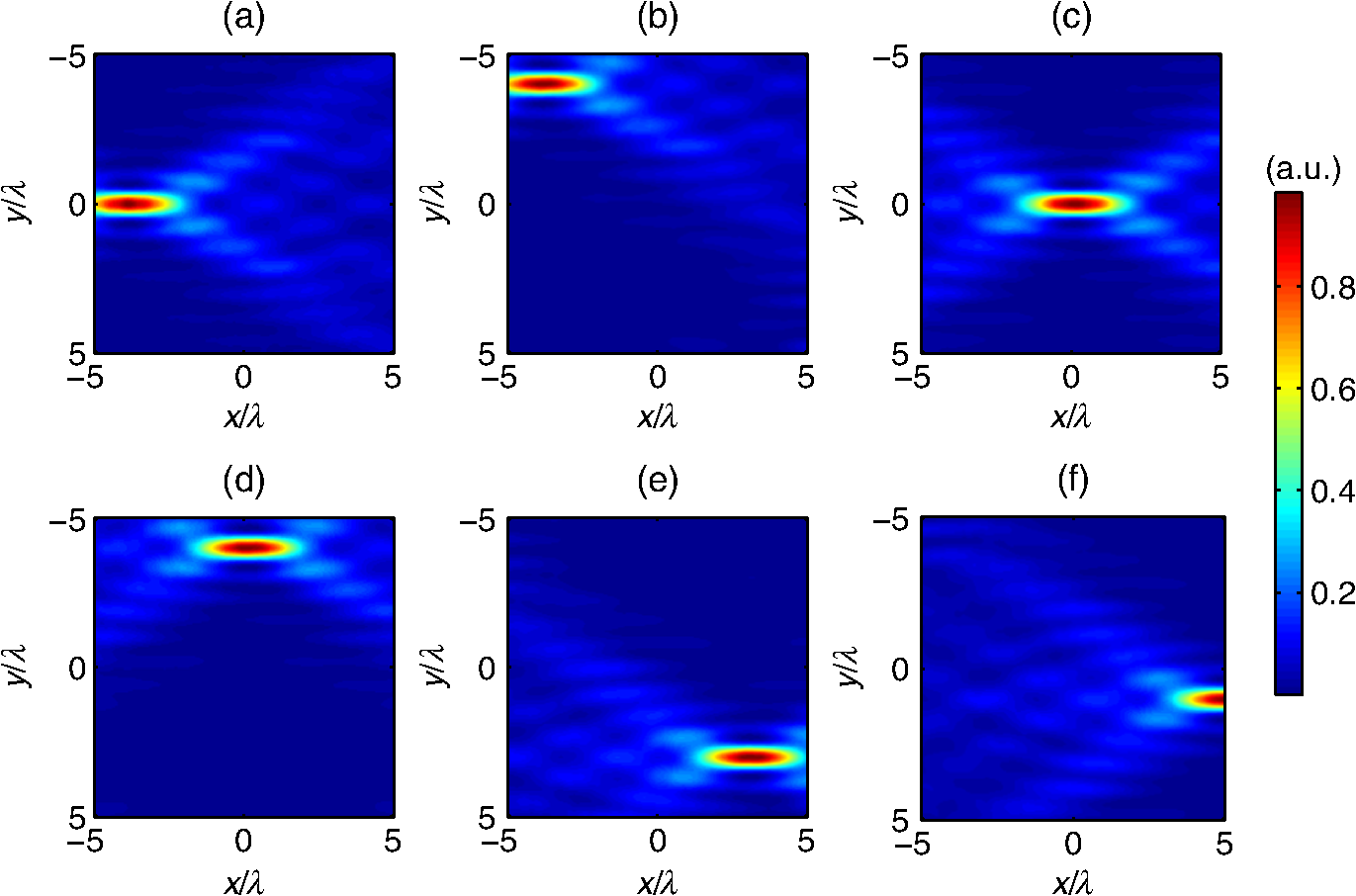$\lambda /20$.

3.3.

Scanning Through Scattering Media

In this section, a simulation quite similar to the one performed in the previous section is investigated. However, in this case, the medium is not homogeneous but consists of cylindrical scatterers with refractive index of 1.45 suspended in water ($n=1.33$). The volume concentration of the scatterers is 30%, which gives a mean free path of 6.9 μm assuming independent scattering. The beam is first scanned in the $x$-direction to show the change in the focal shape and intensity in relation to the depth of the precalculated focus of the beam in the sample (Fig. 6). Second, a simulation is presented for the scanning in the $y$-direction to show that the same principle works in this case as well (Fig. 7). Also, the intensity of the electric fields that are being shown are not only the incident light, rather they are the intensity of the sum of the incident and the scattered electric fields. We mention this because in Fig. 6, as expected, the focused beam is distorted after propagating through the scatterers. But even before the beam reaches the scatterers, the beam is somehow distorted. This is because of the back-scattered light which interacts with the beam. The intensity in Figs. 6 and 7 is normalized to the maximum intensity of the incident nonscattered focused beam. It can be noticed that in Fig. 6(d), the intensity is increased above 1. This is due to the high constructive interference of the near fields between the two cylinders in the vicinity of the focus. Also, it is interesting to note that the supposed position of the focus diverges from the actual position of the focus especially for the deeper foci. This displacement is partly caused by the different speeds of the beam inside and outside the scatterers since the expected focus positions are calculated with the assumption of no scattering. By examining Fig. 6, it becomes apparent that the deeper the light propagates through the sample, the more the intensity of the focus decreases and its shape is distorted. More precisely, the relative width of the beam is enlarged and, in addition, further unintentional “foci” due to interference of scattered light appear at larger depths of the precalculated focus position. We note that to reach these conclusions, it was necessary to run the simulation for more realizations of the scatterers’ positions (figure not shown).

Fig. 6

The normalized intensity of the $E_z$ component of the electric field for axial scanning ($x$-direction) at $y_0=0$. The normalization is relative to the maximum intensity of the incident nonscattered focused beam. The figures from (a) to (f) show focus positions at: ($x_0/\lambda =-8$, $y_0/\lambda =0$), ($x_0/\lambda =-6$, $y_0/\lambda =0$), ($x_0/\lambda =-2$, $y_0/\lambda =0$), ($x_0/\lambda =2$, $y_0/\lambda =0$), ($x_0/\lambda =4$, $y_0/\lambda =0$), and ($x_0/\lambda =9$, $y_0/\lambda =0$). Twenty-one plane waves are used to form the beam. The scatterers are cylinders with refractive index of 1.45, while the surrounding medium has a refractive index of 1.33. The wavelength of the incident light is 1 μm and the maximum divergence angle of the focused beam is 45 deg. The spatial resolution in the FDTD simulation is equal to 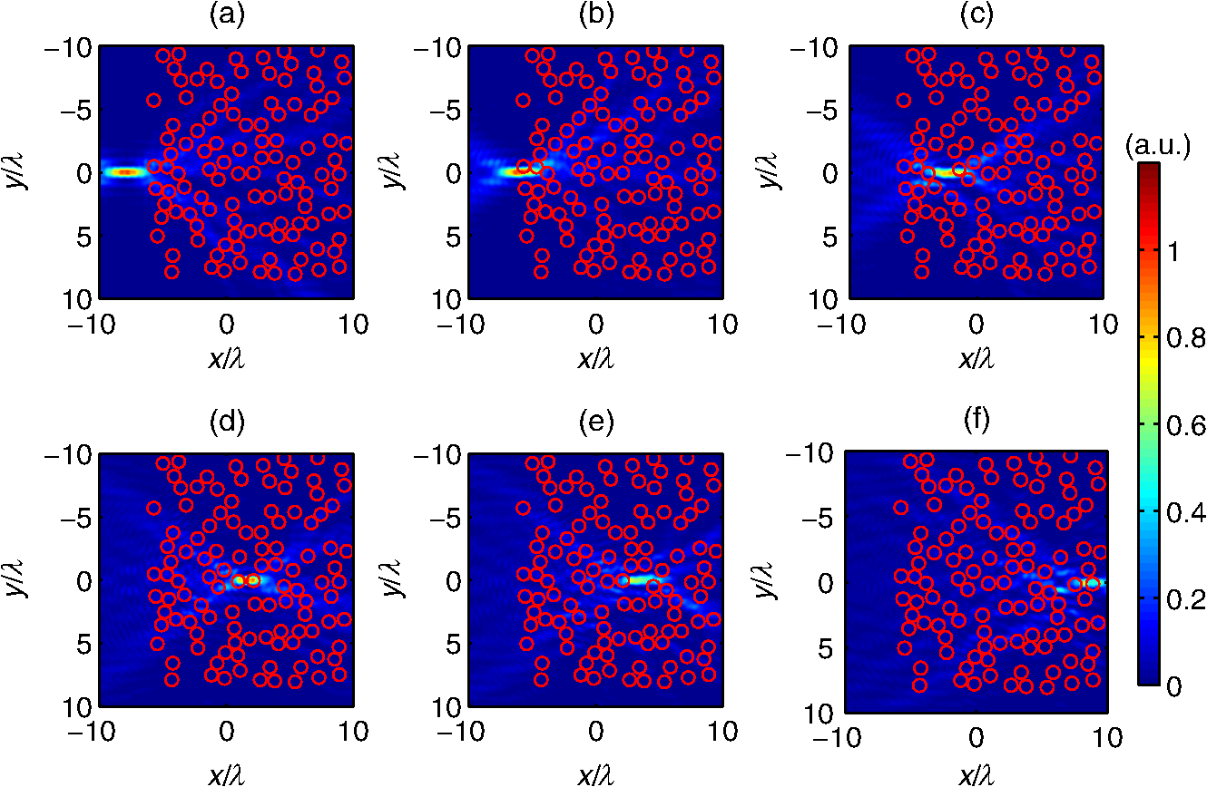$\lambda /20$.

Fig. 7

The normalized intensity of the $E_z$ component of the electric field for lateral scanning ($y$-direction) at $x_0=0$. The normalization is relative to the maximum intensity of the incident nonscattered focused beam. The figures from (a) to (f) show focus positions at: ($x_0/\lambda =-10$, $y_0/\lambda =2$), ($x_0/\lambda =0$, $y_0/\lambda =-8$), ($x_0/\lambda =0$, $y_0/\lambda =-4$), ($x_0/\lambda =0$, $y_0/\lambda =0$), ($x_0/\lambda =0$, $y_0/\lambda =-4$), and ($x_0/\lambda =0$, $y_0/\lambda =8$). Twenty-one plane waves are used to form the beam. The scatterers are cylinders with refractive index of 1.45, while the surrounding medium has a refractive index of 1.33. The wavelength of the incident light is 1 μm, and the maximum divergence angle of the focused beam is 45 deg. The spatial resolution in the FDTD simulation is equal to $\lambda /20$.

The simulations presented in Fig. 6 were allocated a memory of 47.3 Mbyte, compared to 2.25 Mbyte, which is needed to save the data in a classical FDTD simulation. In return, the simulation took $\sim 40\min$ compared to 14 h, which is the time needed for a classical FDTD simulation.