|
|
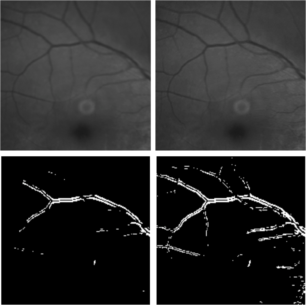
1.IntroductionBlur is one of the main image quality degradations in eye fundus imaging, which along with other factors such as nonuniform illumination or scattering, hinder the clinical use of the images. Its main causes are inherent optical aberrations in the eye, relative camera-eye motion, and improper focusing. Eye motion is related to the patient inability to steady fixate a target in the fundus camera. Many patients have difficulty in fixating, like many elderly patients or those that suffer from amblyopia.1 Because the optics of the eye is part of the optical imaging system, the aberrations of the eye are a common source of image quality degradation. To overcome this limitation, adaptive optics techniques have been successfully applied to correct the aberrations, thus producing high resolution images.2 However, most commercial fundus cameras compensate for spherical refractive errors, but not for astigmatism3—let alone higher-order aberrations. In general, the aberrations of the eye have a stronger impact in image degradation than the aberrations introduced by the rest of the optical system, i.e., the retinal camera. Besides, even though it is possible to measure the optical quality of the camera, it would be exceptional to have readily available additional information related to the optical quality of the patient’s eye. The described scenario is commonplace in the clinical setting, for which we assume the same conditions here. This brings about the need for a restoration procedure that accounts for the lack of information related to the origin of the image degradation. The technique for recovering an original or unblurred image from a single or a set of blurred images in the presence of a poorly determined or unknown point-spread function (PSF) is called blind deconvolution. Removing blur from a single blurred image is an ill-posed problem as there are more unknowns (image and blur) than equations. Having more than one image of the same scene better poses the problem. In retinal imaging, it is not difficult to obtain a second image from the same eye, with the convenience that acquisition conditions remain quite similar. In fact, in Ref. 4, we took advantage of this condition and proposed a blind deconvolution method to restore blurred retinal images acquired with a lapse of time, even in the case where structural changes had occurred in the images. In that work, we detected structural changes, which in turn have clinical relevance, and applied a masking operator so that the images would comply with the considered degradation model. This enabled the successful restoration of many degraded retinal images coming from patient follow-up visits. However, the method is limited to images blurred uniformly; in other words, we assumed the blur to be space-invariant. In Sec. 4.2, we show an attempt at restoring an image degraded with spatially variant blur with this approach. The space-invariant assumption is commonplace in most of the restoration methods reported in the literature,5 but in reality it is a known fact that blur changes throughout the image.6 In this work, we consider the blur to be both unknown and space-variant (SV). This in itself is a novel approach in retinal imaging; relevant to such extent that many common eye related conditions, such as astigmatism, keratoconus, corneal refractive surgery, or even tear break-up, may contribute significantly to a decline in image quality7,8 typically in the form of an SV degradation. An example of such a condition is shown in Fig. 1(a). The image corresponds to an eye from a patient with corneal abnormalities that lead to a loss in visual acuity and a quality degradation of the retinal image [Fig. 1(b)]. Fig. 1(a) Top: Eye with corneal defects that induce retinal images with space-variant (SV) degradation. Bottom: zoomed region. (b) Left column: original image and details. Right column: restored image with proposed approach and details. 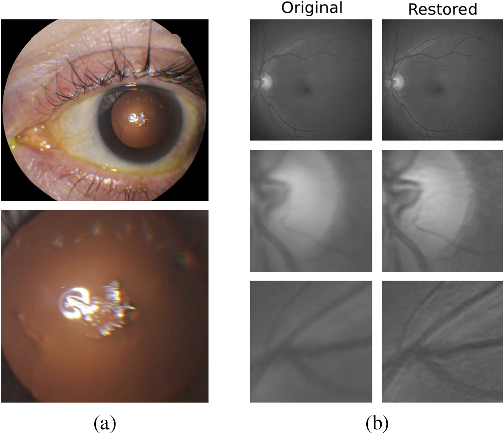 Restoration of images with SV blur from optical aberrations has been reported in the literature,9 although the main limitation is that the blurred image is often restored in regions or patches, which are then stitched together. This inevitably leads to ringing artifacts associated with frequency-domain filtering like in Wiener filtering. Another clear disadvantage is a significant complexity for accurately estimating the SV PSF, for instance Bardsley et al.10 use a phase-diversity based scheme to obtain the PSF associated with an image patch. This type of approach is common in atmospheric optics where the conditions and setup of the imaging apparatus (typically a telescope) are well known and calibrated. Unfortunately, this is not immediately applicable to retinal imaging, at least nonadaptive optics retinal imaging. Recently, there have been several works11–13 that try to solve the SV blind deconvolution problem from a single image. The common ground in these works is that the authors assume that the blur is only due to camera motion. They do this in order to reduce the space in which to search for SV blurs. Despite their approach being more general, the strong assumption of camera motion is simply too restrictive to be applied in the retinal imaging scenario. 1.1.ContributionIn this work, we propose a method for removing blur from retinal images. We consider images degraded with SV blur, which may be due to factors like aberrations in the eye or relative camera-eye motion. Because restoring a single blurred image is an ill-posed problem, we make use of two blurred retinal images from the same eye fundus to accurately estimate the SV PSF. Before the PSF estimation and restoration stages take place, we preprocess the images to accurately register them and compensate for illumination variations not caused by blur, but by the lighting system of the fundus camera. This is depicted in the block diagram shown in Fig. 2. The individual stages of the method are explained in Sec. 3. Fig. 2Block diagram illustrating the proposed method. is the degraded image, is an auxiliary image of the same eye fundus used for the point-spread function (PSF) estimation, and is the restored image. The other variables are intermediate outputs of every stage; their meaning is given in the text.  We assume that in small image patches, the SV blur can be approximated by a spatially invariant PSF. In other words, that in a small region, the wavefront aberrations remain relatively constant; the so-called isoplanatic patch.6 An important aspect of our approach is that instead of deblurring each patch with its corresponding space-invariant PSF—and later stitching together the results—we sew the individual PSFs by interpolation and restore the image globally. This is intended to reduce some artifacts that otherwise would likely appear at the seams of the restored patches. The estimation of the local space-invariant PSFs may fail in patches with hardly any structural information (e.g., such as blood vessels). These poorly estimated or nonvalid PSFs introduce artifacts in the restored image. Detecting such artifacts and inferring the nonvalid PSFs is a difficult problem. Recently, Tallón et al.14 developed a strategy for detecting these patches in an SV deconvolution and denoising algorithm from a pair of images acquired with different exposures: a sharp noisy image with a short exposure and a blurry image with a long exposure. Because they had two distinct input images that were able to: (i) Identify patches where the blur estimates were poor based on a comparison (via a thresholding operation) of the deconvolved patches with the sharp noisy patches. (ii) In those patches, instead of correcting the local PSFs and deconvolving the patches again, they performed denoising in the noisy sharp image patch. The end result is a patchwork-image of deconvolved patches stitched together with denoised patches. Their method is mainly oriented at motion blur, this is the reason for a dual exposure strategy. This is not readily implementable in the retinal imaging scenario where the SV blur is generally caused by factors like aberrations, including those belonging to the patient’s eye optical system, the eye fundus shape, and the retinal camera. In this paper, we address the question “how to identify PSF estimation failure to improve the SV deconvolution of retinal images?” Retinal imaging provides a constrained imaging scenario from which we can formulate a restoration approach that incorporates prior knowledge of blur through the optics of the eye. The novelty in our approach is in the strategy based on eye-domain knowledge for identifying the nonvalid local PSFs and replacing them with appropriate ones. Even though methods for processing retinal images in a space-dependent way (like locally adaptive filtering techniques15,16) have been proposed in the literature; to the best of our knowledge, this is the first time a method for SV deblurring of retinal images is proposed. 2.SV Model of BlurIn our previous work,4 we modeled the blurring of a retinal image by convolution with a unique global PSF. This approximation is valid as long as the PSF changes little throughout the field of view (FOV). In other words, that the blurring is homogenous. In reality, we know that the PSF is indeed spatially variant,6 to such an extent that in some cases the space-invariant approach completely fails, bringing forth the need for an SV approach. To address this limitation, in this work, we model the blurred retinal image by the linear operation where is the unblurred retinal image and is the SV PSF. The operator is a generalization of standard convolution where is now a function of four variables. We can think of this operation as a convolution with a PSF that is now dependent on the position in the image. Standard convolution is a special case of Eq. (1), where for an arbitrary position . Note that the PSF is a general construct that can represent other complex image degradations which depend on spatial coordinates, such as motion blur, optical aberrations, lens distortions, and out-of-focus blur.2.1.Representation of SV PSFAn obvious problem of spatially varying blur is that the PSF is now a function of four variables. Except trivial cases, it is hard to express it by an explicit formula. Even if the PSF is known, we must solve the problem of a computationally efficient representation. In practice, we work with a discrete representation, where the same notation can be used but with the following differences: the PSF is defined on a discrete set of coordinates, the integral sign in Eq. (1) becomes a sum, operator corresponds to a sparse matrix and to a vector obtained by stacking the columns of the image into one long vector. For example in the case of standard convolution, is a block-Toeplitz matrix with Toeplitz blocks and each column of corresponds to the same kernel .17 In the SV case that we address here, as each column of corresponds to a different position , it may contain a different kernel . In retinal imaging, all typical causes of blur change in a continuous gradual way,18 which is why we assume the blur to be locally constant. Therefore, we can make the approximation that locally the PSFs are space-invariant. By taking advantage of this property, we do not have to estimate local PSFs for every pixel. Instead, we divide the image into rectangular windows and estimate only a small set of local PSFs [see Fig. 3(a)] following the method described in Ref. 4 and outlined in Sec. 3. The estimated PSFs are assigned to the centers of the windows from where they were computed. In the rest of the image, the PSF is approximated by bilinear interpolation from the four adjacent local PSFs. This procedure is explained in further detail in the following section. 3.Description of the MethodIn this section, we describe the different stages of the proposed restoration method shown in Fig. 2. This paper follows Ref. 4 but addresses a more general problem: restoration of retinal images in the presence of an SV PSF. In Ref. 4, we showed that the single image blind deconvolution for blurred retinal images does not provide a suitable restoration. Moreover, in images with SV blur, the restoration is even worse. Alternatively, by taking two images of the same retina we can use a multichannel blind deconvolution strategy that is mathematically better-posed.19 In this paper, the estimation of the SV PSF is carried out via local multichannel deconvolution. To illustrate the method and to study its dependence on its tunable parameters, we use an original real image of the retina and obtain two artificially degraded versions from it, denoted by and . Figure 3(a) contains image . The degraded images and have been obtained by blurring the original image with an SV PSF represented by the grid of local PSFs shown in Fig. 3(b) and adding Gaussian zero-mean noise (). The PSF grid was built with realistic PSFs estimated from real blurred retinal images using the method of Ref. 4. 3.1.PreprocessingBecause we use a multichannel scheme for the estimation of the local PSFs, the images are preprocessed so that they meet the requirements imposed by the space-invariant convolutional model given by Eq. (2). This consists in registering the images and adjusting their illumination distribution following Ref. 4. By carrying out this procedure, the remaining radiometric differences between the images are assumed to be caused by blur and noise. Unlike the case considered in Ref. 4, where a relatively long lapse of time between the two image acquisitions may possibly involve a potential structural change, in this study, both the images and are originated from the same image or, in practice, they are acquired one shortly after the other. Therefore, no structural change is expected. Since image is registered and its illumination matched to , we denote this transformed auxiliary image as . 3.2.Estimation of the Local PSFsIn Sec. 2, we described the model for a spatially varying blur in which we assume the PSF to vary gradually, which means that within small regions the blur can be locally approximated by convolution with a space-invariant PSF. For this reason, we approximate the global function from Eq. (1) by interpolating local PSFs estimated on a set of discrete positions. The main advantage of this approach is that the global PSF needs not be computed on a perpixel basis which is inherently time-consuming. The procedure for estimating the local PSFs is the following. We divide the images and with a grid of patches [Fig. 3(a)]. In each patch , we assume a convolutional blurring model where an ideal sharp patch originates from two degraded patches and (for ). The local blurring model is where * is the standard convolution and and are the convolution kernels or local PSFs. The noise ( and ) is assumed to have a constant spectral density and a zero-mean Gaussian distribution of amplitude. Despite the fact that this may not be the most accurate representation of the noise, because the retinal images considered here are acquired by illuminating with a flash, the resulting signal-to-noise ratio is high enough that in the estimation of the PSFs, the impact of noise is not significant.From this model, we can estimate the local PSFs with an alternating minimization procedure as described in Ref. 4 but applied locally. The general guideline is that the patch size should be large enough to include retinal structures and much larger than the size of the local PSF. In Sec. 4, we show further analysis on the robustness of the method to these parameters. Every local PSF is computed on each patch by minimizing the functional with respect to the ideal sharp patch and the blur kernels and . The blur kernel is an estimate of , where is the center of the current window , and is the norm. The first and second terms of Eq. (3) measure the difference between the input blurred patches ( and ) and the sharp patch blurred by kernels and . This difference should be small for the correct solution. Ideally, it should correspond to the noise variance in the image. Although is a restored patch, note that it is not used by our method, but discarded. This is because our method does not work by performing local deconvolutions and sewing restored patches together, which in practice would produce artifacts on the seams. Instead, we perform a global restoration method explained in Sec. 3.5. The two remaining terms of Eq. (3) are regularization terms with positive weighting constants and , which we have set following the fine-tuning procedure described in Ref. 4. The tuning procedure consists of an optimization process where an artificially degraded retinal image is restored by varying and measuring a restoration error. This way an optimal is obtained. Typical values are and . The third term is the total variation of . It improves stability of the minimization and from a statistical perspective, it incorporates prior knowledge about the solution. The last term is a condition linking the convolution kernels which also improves the numerical stability of the minimization. The functional is alternately minimized in the subspaces corresponding to the images and the PSFs. The estimated PSFs for the artificially degraded [Fig. 3(a)] image are shown in Fig. 6(a).3.3.Identifying and Correcting Nonvalid PSFs3.3.1.Strategy based on eye-domain knowledgeThe local PSF estimation procedure does not always succeeds. Consequently, such nonvalid PSFs must be identified, removed, and replaced. In our case, we replace them by an average of adjacent valid kernels. The main reason why the PSF estimation may fail is due to the existence of textureless or nearly homogenous regions bereft of structures with edges (e.g., blood vessels) to provide sufficient information.14 To identify these nonvalid PSFs, we devised an eye-domain knowledge strategy. The incorporation of proper a priori assumptions and domain knowledge about the blur into the method provides an effective mechanism for a successful identification of poorly estimated PSFs. The optics of the eye is part of the imaging system, therefore it is reasonable to assume that the PSF of the imaging system is determined by the PSF of the eye. The retinal camera can indeed be close to diffraction limited with a very narrow PSF, but the optics of the eye is governed by optical aberrations that change across the visual field18 that lead to an SV PSF. The typical PSFs of the human eye, as reported in the literature,18,20 display distinct shapes in many cases displaying long tails’ evidence of the inherent optical aberrations. What is common to all PSFs of the human eye is that the energy is spread from a central lobe and decreases outwardly. In this paper, we assume that PSFs that do not follow this general pattern are nonvalid PSFs which correspond to patches where the estimation failed. In order to prove this, we designed an artificial experiment where we compare the estimated PSFs with the ground-truth PSFs by using a kernel similarity measure proposed by Hu and Yang.21 The measure is based on the peak of the normalized cross correlation between the two PSFs. The authors showed in the paper that this measure is more accurate than the root mean square error, especially because it is shift invariant. The measure is defined as the blur kernel similarity of two kernels, and , where is the normalized cross-correlation function and is the possible shift between the two kernels. Let represent element coordinates, is given by where is the -norm. Larger similarity values reflect more accurate PSF estimation, thus better image restoration. The graphical representation of the similarity measure is shown in Fig. 4(a). The darkest squares correspond to PSFs with the lowest similarity score.Fig. 4(a) PSF similarity measure. (b) Characterization of estimated local PSFs by energy distribution. Histograms plotted in white bars in (b) have been labeled as valid PSFs based on the histogram probability descriptor () described in the text.  The way we determine a nonvalid PSF is by characterizing the energy distribution along the local PSF space. We add the PSF values along concentric squares of radius to build an energy distribution histogram , which is normalized to sum to 1. In Fig. 4(b), we show the histograms for the energy distribution characterization of the estimated PSFs from the artificially degraded retinal image [Fig. 3(a)]. To identify nonvalid PSFs, i.e., PSFs that do not follow the pattern we have previously described, we compute a shape descriptor for defined as the probability , where is the mode of . This descriptor gives an indication of how much a histogram is spread in relation to the peak () of the histogram. Particularly, it yields low values when the mode is located in the first few bins of the histogram and large values otherwise. This descriptor can be correlated with the PSF similarity measure to determine how it discriminates valid and nonvalid PSFs.In Fig. 5, we plot the similarity measure against for the estimated PSFs from two different retinal images which have been artificially degraded. The correlation coefficient for the two variables is . In addition to the correlation, from the plot we note that most PSFs with high have low kernel similarity () values, which is an indication that these are nonvalid or poorly estimated PSFs. A machine learning algorithm or clustering technique that automatically classifies nonvalid PSFs is out of the scope of this paper. Instead, our aim is to show that the energy characterization approach is sufficient to identify nonvalid PSFs, even at the expense of a few valid ones. As we show in Sec. 4.1, this is not critical because the PSF changes smoothly throughout the FOV. Fig. 5PSF similarity measure () versus histogram probability (). An value of 1 represents an accurately estimated kernel. Low values are associated with correctly estimated kernels.  The histograms plotted in white bars in Fig. 4(b) correspond to PSFs with , which we have labeled as valid PSFs. This means that we are favoring histograms skewed toward the left side. This is based on our assumption of the pattern that valid PSFs should follow. This correlates well with the similarity measure. Note that most PSFs with low similarity measure [darkest squares in Fig. 4(a)] have been correctly identified as nonvalid PSFs [black histograms in Fig. 4(b) and PSFs labeled with boxes in Fig. 6(a)]. Fig. 6(a) Estimated set of local PSFs. (b) New set of local PSFs with nonvalid PSFs replaced [compared with ground-truth set Fig. 3(b)]. Nonvalid PSFs have been labeled with a red square. 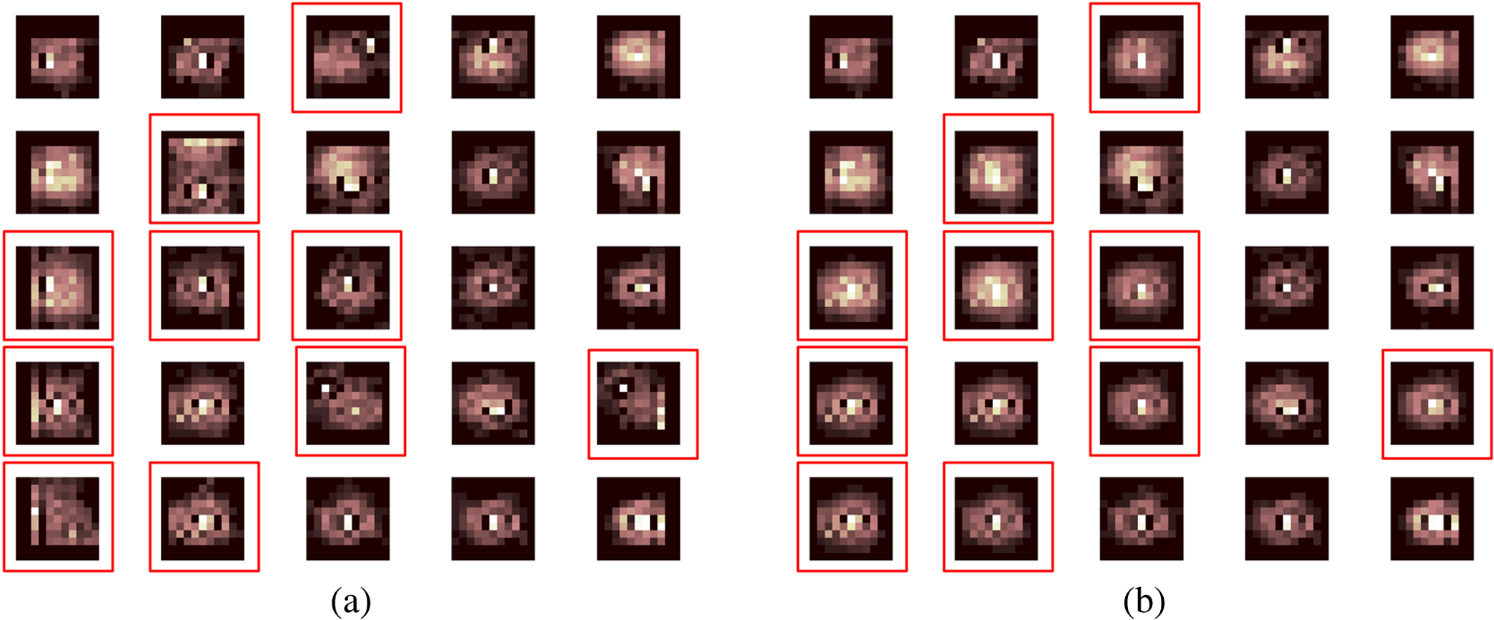 The procedure for correcting the nonvalid local PSFs consists of replacing them with the average of adjacent valid kernels. Without this correction, the reconstruction develops ringing artifacts [see for example Fig. 11(b)]. The new set of valid local PSFs after replacing the nonvalid ones for the artificially degraded image is shown in Fig. 6(b). 3.4.PSF InterpolationThe computation of the SV PSF is carried out by interpolating the local PSFs estimated on the regular grid of positions. The PSF values at intermediate positions are computed by bilinear interpolation of four adjacent known PSFs,22 as shown in Fig. 7. Indexing any four adjacent grid points as (starting from the top-left corner and continuing clockwise), the SV PSF in the position between them is defined as where is the coefficients of bilinear interpolation. Let us denote and as minimum and maximum -coordinates of the subwindow, respectively. Analogously, and are the -coordinates. Using auxiliary quantities the bilinear coefficients areFig. 7Because the blur changes gradually, we can estimate convolution kernels on a grid of positions and approximate the PSF in the rest of the image (bottom kernel) by interpolation from four adjacent kernels.  In light of the definition for an SV PSF in Eq. (7), we can compute the convolution of Eq. (1) as a sum of four convolutions of the image weighted by coefficients In the same fashion, the operator adjoint to (SV counterpart of correlation) denoted by can also be defined in terms of the sums of four convolutions weighted by the coefficients. These two operators are needed in all first-order minimization algorithms as the one used in the restoration stage (see Ref. 23 for further details). 3.5.RestorationHaving estimated a reliable SV PSF, we proceed to deblur the image. Image restoration is typically formulated within the Bayesian paradigm, in which the restored image is sought as the most probable solution to an optimization problem. The restoration can be described as the minimization of the functional where is the blurred observed image, is the blurring operator [Eq. (1)], is the unknown sharp image, and is a positive regularization constant, which we have set according to a fine-tuning procedure.4 The tuning procedure consists in artificially degrading a retinal image and restoring it with Eq. (14) by varying . Because the sharp original image is known we can compare it against the restored image using a metric like the peak-signal-to-noise ratio to determine an optimal value of . The first term penalizes the discrepancy between the model and the observed image. The second term is the regularization term which serves as a statistical prior. As regularization we use total variation, a technique that exploits the sparsity of image gradients in natural images. At present, solving the convex functional of Eq. (14) is considered a standard way to achieve close to state-of-the-art restoration quality without excessive time requirements.24 We used an efficient method25 to solve Eq. (14) iteratively as a sequence of quadratic functionalsThe functional of Eq. (15) bounds the original function in Eq. (14) and has the same value and gradient in the current , which guarantees convergence to the global minimum. To solve Eq. (15), we used the conjugate gradient method.17 The initial value of for is set to be equal to . In order to avoid numerical instability for areas with small gradient ( approaching zero), we use a relaxed -form of the minimized functional in Eq. (14), which implies that is equal to . As regards the restoration of color RGB retinal images, we consider the following. The most suitable channel for PSF estimation is the green because it provides the best contrast.26 This is mainly due to the spectral absorption of the blood in this band, which yields the dark and well contrasted blood vessels.27 Conversely, the blue channel encompasses the wavelengths most scattered and absorbed by the optical media of the eye,28 therefore the image in this band has very low energy and a relatively high level of noise. In the spectral zone of wavelengths larger than 590 nm, the light scattering on the red blood cells and the light reflection from the eye structures behind the vessel are dominant.29 This produces the red band to be saturated and of poor contrast. As a result, we estimate the SV PSF from the green channel of the RGB color image, and later deconvolve every R, G, and B channels with the estimated SV PSF to obtain a restored RGB color image. 4.Experiments and ResultsWe performed several experiments on artificially and naturally degraded images to illustrate the appropriateness of the SV approach for restoring blurred retinal images. Moreover, to achieve an artifact-free restoration, we used our strategy for detecting and replacing the nonvalid local PSFs. 4.1.Artificially Degraded ImagesFor the artificial experiment, we take a pair of images and degrade them with a grid of realistic PSFs plus Gaussian noise (). The grid of PSFs was built upon realistic PSFs estimated from real degraded retinal images following the approach of Ref. 4. From the two input images, we restore one, and the other is used exclusively for the purpose of PSF estimation. We estimate the local PSFs by dividing the image into overlapping patches on a grid [as shown in Fig. 3(a)]. The estimated PSFs are shown in Fig. 6(a). Because the PSF estimation may fail, we identify the nonvalid PSFs as described in Sec. 3.3. We replace them with with the average of adjacent valid kernels. In Fig. 8(a), we show the restored artificial image with the directly estimated PSFs. The effect of nonvalid PSFs is evident in the poor quality of the restoration and the ringing artifacts. In Fig. 8(b), we show the restoration with the proposed method, where the nonvalid PSFs have been identified, removed, and replaced by the average of adjacent PSFs. To evaluate the restoration, we use the cumulative error histogram on a patch basis. The error5 is the difference between a recovered image with the estimated kernels and the known ground-truth sharp image over the difference between the deblurred image with the ground-truth kernels. The error is given by . In Fig. 8(c), we show the cumulative error histogram for three restorations. H1 is the restoration with the directly estimated PSFs. It is important to note that shifted local PSFs warp the image which introduce additional artifacts and is the reason for such a low performance with approximately 40% of patches with an error lower than 2.5. After shifting the centroid of the PSFs to the geometrical center [restoration H2 in Fig. 8(c)], the reconstruction error is reduced significantly, about 60% of patches have an error lower than 1.5. Finally, the restoration (H3) with the removal of nonvalid PSFs increases significantly with all patches now displaying an error lower than 1.5. This means that after the nonvalid PSFs have been replaced the restoration quality is significantly increased. Fig. 8(a) Restoration with the set of directly estimated PSFs shown in Fig. 6(a) (notice the artifacts due to nonvalid PSFs) and (b) restoration with the new set of PSFs with nonvalid PSFs replaced shown in Fig. 6. (c) Error histogram for evaluating the reconstruction using: H1—directly estimated PSFs, H2—PSFs shifted toward the geometrical center, and H3—the new set of valid PSFs.  To determine the limitations and robustness of the proposed method, we carried out several tests. First, we need to determine an optimal patch size for accurately estimating the local PSF. A patch that is too small compared to the kernel size may not have enough information and is likely to favor the trivial solution (convolution with a delta). Conversely, a patch that is bigger than necessary may hinder the SV approach in addition to increasing the computational burden. In Fig. 9(a), we show the mean similarity measure versus the image patch size. It is important to note that a patch size of roughly four times the kernel size may be sufficient for an accurate PSF estimation. Increasing too much the patch size hinders the PSF estimation. Fig. 9(a) Mean similarity measure versus patch size. (b) Mean reconstruction error versus local PSF size. (c) Reconstruction error versus PSF grid size.  The second aspect to consider is under- and over-estimation of the local PSF size. In Fig. 9(b), we show the mean patch reconstruction error versus PSF size. As expected the error is minimum when the size is similar to the true size, yet under-estimating the PSF size is worse than over-estimating. In relation to the SV characterization of the blur, we performed the PSF estimation with a different number of kernels. Initially with a coarse grid increasing up to a fine grid (the grid is the ground-truth). A similar behavior is observed. Under-estimating the proper PSF grid size has a negative effect in that the SV nature of the blur is hardly identified which yields an error above 6 for the whole image. In this case, the error is not computed on a patch-basis because of the variable grid size. 4.2.Naturally Degraded ImagesAll of the naturally degraded images used in the experiments were acquired in pairs, typically with a time span between acquisitions of several minutes. Initially, to show the limits of the space-invariant approach we restored the blurred retinal image from Fig. 10(a) with a single global PSF with the space-invariant method we proposed in Ref. 4. This image corresponds to the eye fundus of a patient with strong astigmatism, which induces an SV blur as depicted by the image details shown in Figs. 10(b)–10(e). The restoration is shown in Fig. 11(a) and we can clearly observe various artifacts despite an increase in sharpness in a small number of areas. In view of this, it is evident that the space-invariant assumption does not hold in such cases. In the following, we move to the SV approach. Fig. 10(a) Retinal image degraded with real SV blur given by strong astigmatism. (b), (c), (d), and (e) zoomed regions to show the SV nature of the blur. 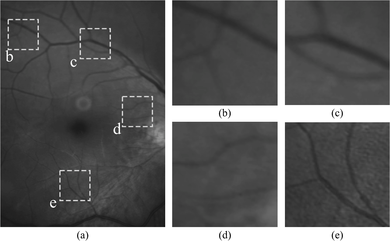 Fig. 11(a) Space-invariant restoration, (b) SV restoration with directly estimated PSFs, and (c) SV restoration with the new set of PSFs. The reader is strongly encouraged to view these images in full resolution at http://www.goapi.upc.edu/usr/andre/sv-restoration/index.html.  To carry out the SV restoration, we estimated the local PSFs on a grid of image patches. From the estimated PSFs shown in Fig. 12(a), we notice a clear variation in shape mainly from the top-right corner where they are quite narrow, to the bottom left corner where they are more spread and wide. This variation is consistent with the spatial variation of the blur observed in the retinal image of Fig. 10(a). We restored the image with these local PSFs that were estimated directly without any adjustment. The restored image is shown in Fig. 11(b). One immediately obvious feature is that in several areas the restoration is rather poor, displaying ringing artifacts, whereas in others it is to some extent satisfactory. The local poor-restoration is linked to areas where the PSF estimation failed. By removing and correcting these nonvalid local PSFs, we obtained a noteworthy restoration shown in Fig. 11(c). Notice the overall improvement in sharpness and resolution with small blood vessels properly defined as shown by the image-details in the third column of Fig. 13. It could be said that without the replacement of the nonvalid PSFs the image quality after restoration is certainly worse than the original degraded image (see second column of Fig. 13). Fig. 12(a) Estimated set of local PSFs from naturally degraded retinal image shown in Fig. 10(a). (b) Set of local PSFs after replacing nonvalid PSFs. Nonvalid PSFs have been labeled with a red square.  Fig. 13Details of restoration. From left to right: the original degraded image, the SV restoration without correction of PSFs and the SV restoration with the correction.  To further demonstrate the capabilities of our method, additional restoration results on real cases from the clinical practice are shown in the following figures. As we mentioned in Sec. 1, a typical source of retinal image degradation comes from patients with corneal defects in which the cornea has an irregular structure [Fig. 1(a)]. This induces optical aberrations, which are mainly responsible for the SV blur observed in the retinal image. The image details shown in Fig. 1(b) reveal a significant improvement in which the retinal structures are much sharper and enhanced. In Fig. 14(a), a full color retinal image is shown, in which three small hemorrhages are more easily discernible in the restored image, along with small blood vessels. Another retinal image, shown in Fig. 14(b), reveals a clear improvement in resolution with a much finer definition of blood vessels. Fig. 14Other retinal images restored with the proposed method. (a) First row: original and restored full-size retinal images. (b) Second and third rows: image details.  In addition, we processed retinal angiography images to test our method against a different imaging modality. Ocular angiography is a diagnostic test that documents, by means of photographs, the dynamic flow of dye in the blood vessels of the eye.30 The ophthalmologists use these photographs both for diagnosis and as a guide to patient treatment. Ocular angiography differs from fundus photography in that it requires an exciter–barrier filter set (for further details see Ref. 30). The retinal angiography shown in Fig. 15 is degraded with a mild SV blur that hinders the resolution of small—yet important—details. The restoration serves to overcome this impediment; this can be observed from the zoomed-detail of the restored image. The image enhancement may be useful for the improvement of recent analysis techniques for automated flow dynamics and identification of clinical relevant anatomy in angiographies.31 Fig. 15Restoration of a retinal angiography. First row: original and restored full retinal images. Second row: image details. 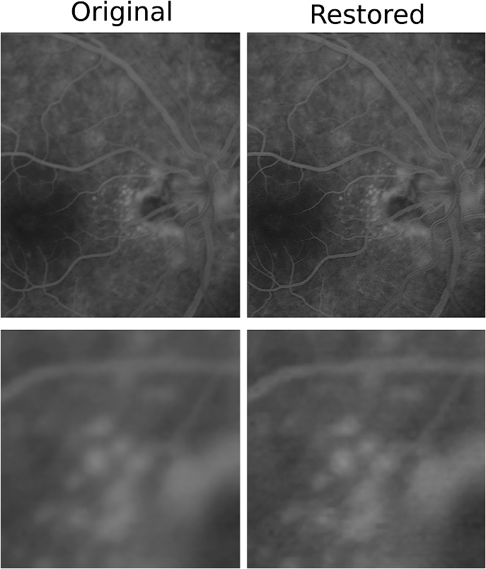 Finally, another way to demonstrate the added value of deblurring the retinal images is to extract important features, in this case detection of blood vessels. Such a procedure is commonly used in many automated disease detection algorithms. The improvement in resolution paves the way for a better segmentation of structures with edges. This is in great part due to the effect of the total variation regularization because it preserves the edge information in the image. To carry out the detection of the retinal vasculature, we used Kirsch’s method.32 It is a matched filter algorithm that computes the gradient by convolution with the image and eight templates to account for all possible directions. This algorithm has been widely used for detecting the blood vessels in retinal images.33 In Fig. 16, we show the detection of the blood vessels from a real image of poor quality image and its restored version using our proposed method. A significant improvement in blood vessel detection is achieved. Smaller blood vessels are detected in the restored image, whereas the detection from the original image barely covers the main branch of the vasculature. 5.ConclusionIn this paper, we have introduced a method for restoring retinal images affected by SV blur by means of blind deconvolution. To do so, we described a spatially variant model of blur in terms of a convolution with a PSF that changes depending on its position. Since the SV degradation changes smoothly across the image, we showed that the PSF need not be computed for all pixels, which is quite a demanding task, but for a small set of discrete positions. For any intermediate position bilinear interpolation suffices. In this way, we achieve an SV representation of the PSF. The estimation of accurate local PSFs proved difficult due to the very nature of the images; they usually contain textureless or nearly homogenous regions that lack retinal structures, such as blood vessels, to provide sufficient information. In this regard, we proposed a strategy based on eye-domain knowledge to adequately identify and correct such nonvalid PSFs. Without this, the restoration results are artifact-prone with an overall image quality that is worse than the original image. The proposal has been tested on artificially and naturally degraded retinal images coming from the clinical practice. The details from the restored retinal images show an important enhancement, which is also demonstrated with the improvement in the detection of the retinal vasculature. In summary, it seems clear that the SV restoration of blurred retinal images is significant enough to leverage the images’ clinical use. Improving the visibility of subtle details like small hemorrhages or small blood vessels may prove useful for disease screening purposes, follow-up monitoring, or early disease detection. With the new challenges faced by clinical services in the 21st century, automated medical image analysis tools are mandatory—this work is a step toward that direction. AcknowledgmentsThis research has been partly funded by the Spanish Ministerio de Ciencia e Innovación y Fondos FEDER (project DPI2009-08879) and projects TEC2010-09834-E and TEC2010-20307. Financial support was also provided by the Grant Agency of the Czech Republic under project 13-29225S. Authors are grateful to Juan Luís Fuentes from the Miguel Servet University Hospital (Zaragoza, Spain) for providing images. The first author also thanks the Spanish Ministerio de Educación for an FPU doctoral scholarship. ReferencesH. BartlingP. WangerL. Martin,
“Automated quality evaluation of digital fundus photographs,”
Acta Ophthalmol., 87
(6), 643
–647
(2009). http://dx.doi.org/10.1111/aos.2009.87.issue-6 ACOPAT 0001-639X Google Scholar
P. Godaraet al.,
“Adaptive optics retinal imaging: emerging clinical applications,”
Optom. Vision Sci., 87
(12), 930
–941
(2010). http://dx.doi.org/10.1097/OPX.0b013e3181ff9a8b OVSCET 1040-5488 Google Scholar
J. ArinesE. Acosta,
“Low-cost adaptive astigmatism compensator for improvement of eye fundus camera,”
Opt. Lett., 36
(21), 4164
–4166
(2011). http://dx.doi.org/10.1364/OL.36.004164 OPLEDP 0146-9592 Google Scholar
A. G. Marrugoet al.,
“Retinal image restoration by means of blind deconvolution,”
J. Biomed. Opt., 16
(11), 116016
(2011). http://dx.doi.org/10.1117/1.3652709 JBOPFO 1083-3668 Google Scholar
A. Levinet al.,
“Understanding blind deconvolution algorithms,”
IEEE Trans. Pattern Anal. Mach. Intell., 33
(12), 2354
–2367
(2011). http://dx.doi.org/10.1109/TPAMI.2011.148 ITPIDJ 0162-8828 Google Scholar
P. Bedggoodet al.,
“Characteristics of the human isoplanatic patch and implications for adaptive optics retinal imaging,”
J. Biomed. Opt., 13
(2), 024008
(2008). http://dx.doi.org/10.1117/1.2907211 JBOPFO 1083-3668 Google Scholar
R. Tuttet al.,
“Optical and visual impact of tear break-up in human eyes,”
Invest. Ophthalmol. Visual Sci., 41
(13), 4117
–4123
(2000). IOVSDA 0146-0404 Google Scholar
J. Xuet al.,
“Dynamic changes in ocular zernike aberrations and tear menisci measured with a wavefront sensor and an anterior segment OCT,”
Invest. Ophthalmol. Vis. Sci., 52
(8), 6050
–6056
(2011). http://dx.doi.org/10.1167/iovs.10-7102 IOVSDA 0146-0404 Google Scholar
T. CostelloW. Mikhael,
“Efficient restoration of space-variant blurs from physical optics by sectioning with modified Wiener filtering,”
Digital Signal Process., 13
(1), 1
–22
(2003). http://dx.doi.org/10.1016/S1051-2004(02)00004-0 DSPREJ 1051-2004 Google Scholar
J. Bardsleyet al.,
“A computational method for the restoration of images with an unknown, spatially-varying blur,”
Opt. Express, 14
(5), 1767
–1782
(2006). http://dx.doi.org/10.1364/OE.14.001767 OPEXFF 1094-4087 Google Scholar
S. HarmelingM. HirschB. Scholkopf,
“Space-variant single-image blind deconvolution for removing camera shake,”
Adv. Neural Inf. Process. Syst., 23 829
–837
(2010). Google Scholar
O. Whyteet al.,
“Non-uniform deblurring for shaken images,”
Int. J. Comput. Vis., 98
(2), 168
–186
(2012). Google Scholar
A. Guptaet al.,
“Single image deblurring using motion density functions,”
in European Conf. on Computer Vision (ECCV 2010),
171
–184
(2010). Google Scholar
M. Tallónet al.,
“Space-variant blur deconvolution and denoising in the dual exposure problem,”
Inf. Fusion, 14
(4), 396
–409
(2012). http://dx.doi.org/10.1016/j.inffus.2012.08.003 Google Scholar
N. SalemA. Nandi,
“Novel and adaptive contribution of the red channel in pre-processing of colour fundus images,”
J. Franklin Inst., 344
(3–4), 243
–256
(2007). http://dx.doi.org/10.1016/j.jfranklin.2006.09.001 JFINAB 0016-0032 Google Scholar
A. G. MarrugoM. S. Millán,
“Retinal image analysis: preprocessing and feature extraction,”
J. Phys.: Conf. Ser., 274
(1), 012039
(2011). http://dx.doi.org/10.1088/1742-6596/274/1/012039 1742-6588 Google Scholar
G. GolubC. Van Loan, Matrix Computations, Johns Hopkins University Press, Baltimore, Maryland
(1996). Google Scholar
R. NavarroE. MorenoC. Dorronsoro,
“Monochromatic aberrations and point-spread functions of the human eye across the visual field,”
J. Opt. Soc. Am. A, 15
(9), 2522
–2529
(1998). http://dx.doi.org/10.1364/JOSAA.15.002522 JOAOD6 0740-3232 Google Scholar
F. SroubekJ. Flusser,
“Multichannel blind deconvolution of spatially misaligned images,”
IEEE Trans. Image Process., 14
(7), 874
–883
(2005). http://dx.doi.org/10.1109/TIP.2005.849322 IIPRE4 1057-7149 Google Scholar
R. Navarro,
“The optical design of the human eye: a critical review,”
J. Optom., 2
(1), 3
–18
(2009). http://dx.doi.org/10.3921/joptom.2009.3 Google Scholar
Z. HuM.-H. Yang,
“Good regions to deblur,”
in European Conf. on Computer Vision (ECCV 2012),
59
–72
(2012). Google Scholar
J. G. NagyD. P. O’Leary,
“Restoring images degraded by spatially variant blur,”
SIAM J. Sci. Comput., 19
(4), 1063
–1082
(1998). http://dx.doi.org/10.1137/S106482759528507X SJOCE3 1064-8275 Google Scholar
M. SorelF. SroubekJ. Flusser,
“Towards super-resolution in the presence of spatially varying blur,”
Super-Resolution Imaging, 187
–218 CRC Press, Boca Raton, Florida
(2010). Google Scholar
P. CampisiK. Egiazarian, Blind Image Deconvolution: Theory and Applications, CRC Press, Boca Raton, Florida
(2007). Google Scholar
A. ChambolleP. L. Lions,
“Image recovery via total variation minimization and related problems,”
Numer. Math., 76
(2), 167
–188
(1997). http://dx.doi.org/10.1007/s002110050258 NUMMA7 0029-599X Google Scholar
A. HooverM. Goldbaum,
“Locating the optic nerve in a retinal image using the fuzzy convergence of the blood vessels,”
IEEE Trans. Med. Imaging, 22
(8), 951
–958
(2003). http://dx.doi.org/10.1109/TMI.2003.815900 ITMID4 0278-0062 Google Scholar
L. GaoR. T. SmithT. S. Tkaczyk,
“Snapshot hyperspectral retinal camera with the Image Mapping Spectrometer (IMS),”
Biomed. Opt. Express, 3
(1), 48
–54
(2012). http://dx.doi.org/10.1364/BOE.3.000048 BOEICL 2156-7085 Google Scholar
M. HammerD. Schweitzer,
“Quantitative reflection spectroscopy at the human ocular fundus,”
Phys. Med. Biol., 47
(2), 179
–191
(2002). http://dx.doi.org/10.1088/0031-9155/47/2/301 PHMBA7 0031-9155 Google Scholar
V. Vuceaet al.,
“Blood oxygenation measurements by multichannel reflectometry on the venous and arterial structures of the retina,”
Appl. Opt., 50
(26), 5185
–5191
(2011). http://dx.doi.org/10.1364/AO.50.005185 APOPAI 0003-6935 Google Scholar
P. SaineM. Tyler, Ophthalmic Photography: Retinal Photography, Angiography, and Electronic Imaging, Butterworth-Heinemann, Woburn, Massachusetts
(2002). Google Scholar
T. Holmeset al.,
“Dynamic indocyanine green angiography measurements,”
J. Biomed. Opt., 17
(11), 116028
(2012). http://dx.doi.org/10.1117/1.JBO.17.11.116028 JBOPFO 1083-3668 Google Scholar
R. A. Kirsch,
“Computer determination of the constituent structure of biological images,”
Comput. Biomed. Res., 4
(3), 315
–328
(1971). http://dx.doi.org/10.1016/0010-4809(71)90034-6 CBMRB7 0010-4809 Google Scholar
M. Al-RawiM. QutaishatM. Arrar,
“An improved matched filter for blood vessel detection of digital retinal images,”
Comput. Biol. Med., 37
(2), 262
–267
(2007). http://dx.doi.org/10.1016/j.compbiomed.2006.03.003 CBMDAW 0010-4825 Google Scholar
BiographyAndrés G. Marrugo received the BE degree (summa cum laude) in mechatronical engineering from the Technological University of Bolívar, Cartagena, Colombia, in 2008, the MSc in photonics, and the PhD in optical engineering from the Technical University of Catalonia, Barcelona, Spain, in 2009 and 2013, respectively. He is currently with the Technological University of Bolívar. He is a member of SPIE, the Spanish Optical Society, and the European Optical Society. María S. Millán received the PhD in physics in 1990 and is a full professor of the College of Optics and Optometry in the Technical University of Catalonia, Barcelona, Spain. Her research work on image processing involves optical and digital technologies, algorithms, and development of new applications to industry and medicine. She has been a representative of the Spanish Territorial Committee in the International Commission for Optics. She is a member of the Optical Society of America, a fellow member of SPIE and a fellow member of the European Optical Society. Michal Šorel received the MSc and PhD degrees in computer science from Charles University in Prague, Czech Republic, in 1999 and 2007, respectively. From 2012 to 2013 he was a postdoctoral researcher at Heriot-Watt University in Edinburgh, Scotland, and the University of Bern, Switzerland. Currently he is a research fellow in the Institute of Information Theory and Automation, Academy of Sciences of the Czech Republic. Filip Šroubek received the MS degree in computer science from the Czech Technical University, Prague, Czech Republic, in 1998 and the PhD degree in computer science from Charles University, Prague, Czech Republic, in 2003. From 2004 to 2006, he was on a postdoctoral position in the Instituto de Optica, CSIC, Madrid, Spain. In 2010 and 2011, he was the Fulbright visiting scholar at the University of California, Santa Cruz. He is currently with the Institute of Information Theory and Automation of the Academy of Sciences of the Czech Republic. |