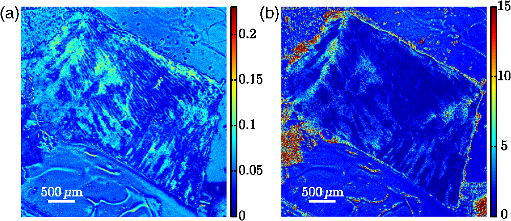
2.1.

Sample Preparation

Tendon tissue was taken from medial femoral condyle of a chicken’s knee, bought fresh from the supermarket. A small section of the tissue was embedded in a mounting medium for cryo-sectioning (O.C.T., Sakura, Alphen aan den Rijn, The Netherlands). Rapid freezing of the O.C.T. embedded tissue was completed using liquid nitrogen. This frozen section was stored in a freezer ($-60°\mathrm{C}$) until cut with a cryostat into 50-μm thin tissue sections. The cutting plane was parallel to the collagen fibers. The thin sections were placed on standard microscope glass slides and stored in a freezer ($-60°\mathrm{C}$). Before being measured, the tissue samples were brought back to room temperature and covered with a standard cover slip. Edges of the cover slip were sealed with Vaseline to avoid dehydration. Between measurements, the slides were stored at 4°C.

2.2.

SHG Imaging

SHG images were collected on a Zeiss LSM 510 meta microscope using a Coherent Mira 900 for excitation at 790 nm. Imaging was done with a $40\times$ 1.2 NA objective. A custom built polarization setup, which compensates for any birefringence in the optical path, was used to ensure circular polarization. The average power at the focal plane was approximately 8.

2.3.

MMI Setup

After the samples were imaged with SHG, they were measured in a custom built MMI ellipsometer, shown in Fig. 1. The system uses ferroelectric liquid crystals for both the polarization state generator and analyzer. Details of the system can be found in Aas et al.²³ An improvement was made to the illumination, by replacing both the laser and rotating diffuser, with a 940 nm collimated light emitting diode (LED). In addition, a motorized rotation stage for the sample was introduced in order to image the sample at the different projections needed to extract the 3-D direction, as described below.

Fig. 1

The Mueller matrix imaging (MMI) setup consisting of the polarization state generator (PSG) and the polarization state analyzer (PSA). P1 and P2 are the linear polarizers, $R1,\dots ,R4$ are the retarders and $F1,\dots ,F4$ are the ferroelectric liquid crystals.

The system was calibrated using the eigenvalue calibration method²⁴ on four reference samples (air, two polarizers, and a retarder), ensuring the correct measurement of the Mueller matrix. By comparing the measurement of air to the identity matrix, an error estimate was made resulting in a measure for the accuracy of the system.

2.4.

Decomposition of the Mueller Matrix

As the differential decomposition method is able to decompose simultaneous polarization effects, it was chosen for the decomposition of the measured Mueller matrices presented here. Due to the measurement noise, some of the measured Mueller matrices are slightly unphysical, which was compensated for by using the filtering described by Cloude,²⁵ prior to the decomposition.

The differential decomposition results in two matrices, $L_m$ and $L_u$,²⁰ where $L_m$ contains the elements used to calculate the retardance and the diattenuation. The uncertainties (standard deviation) in the retardance and the diattenuation can be calculated by using the same matrix elements from $L_u$ as those originally used from $L_m$. Furthermore, the depolarization can be calculated from $L_u$. In this study, the relevant properties are the linear retardance $\delta$, the angle of orientation of the linear retardance $\theta$, and the depolarization $\mathrm{\Delta }$ (It is here noted that the depolarization [${\mathrm{\Delta }}^{\log -M}$, Eq. (19) in the paper by Kumar et al.¹²] has the wrong signs of the exponential, it should be ${\mathrm{\Delta }}^{\log -M}=1-(1/3)(e^{{\alpha }_1}+e^{{\alpha }_3}+e^{{\alpha }_3})$ as discussed in a private correspondence with Ossikovski, one of the authors of the original paper.).¹²

2.5.

Directional Calculation

In every day life, we are familiar with determining the orientation of an object just by looking at it. Because our eyes are separated by a distance, they see two different projections of an object which enables deduction of the object’s orientation. The MMI setup can only image one projection, but it is possible to rotate the sample in two different sample rotations $\alpha$, see Figs. 2 and 3, and then use the two resulting images to calculate the direction of the imaged birefringent structure, i.e., the collagen framework.

Fig. 2

Rotation $\alpha$ of the sample seen from above the setup.

Fig. 3

The coordinate systems used for the calculation of the directions. The laboratory frame $(xyz)$ is identical to the sample frame of reference $(x^{\prime }{y}^{\prime }{z}^{\prime })$ at $\alpha =0$. The $x$-axis points along the illumination direction toward the camera and $z$ is vertical. As the rotation is around $z$, $z^{\prime }=z$ for any $\alpha$. The lower row of figures shows the projection of a three-dimensional (3-D) fiber onto the imaging plane, for different rotations of the sample ($\alpha$).

In order to derive the direction of anisotropic structures, it is convenient to start with the Euler transformations.²⁶ They require the definition of two coordinate systems, the laboratory frame of reference and the sample frame of reference. Let $\mathit{p}=[x,y,z]$ describes a vector in the laboratory frame of reference. The frame of reference is defined in such a way that the $x$-axis points along the direction of illumination, the $y$-axis is horizontal, and the $z$-axis is vertical, see Fig. 2. Let ${\mathit{p}}^{\prime }=[x^{\prime },y^{\prime },z^{\prime }]$ be a vector in the sample frame of reference. The sample frame of reference coincides with the laboratory frame for a rotation $\alpha =0\mathrm{deg}$, see Fig. 2. The sample is only rotated around the $z=z^{\prime }$ axis, see Figs. 2 and 3, resulting in the following Euler rotation matrix

By using this transformation, it is possible to transform from the sample frame of reference ${\mathit{p}}^{\prime }$ to the laboratory frame of reference $\mathit{p}$, by $\mathit{p}=\mathit{R}(-\alpha ){\mathit{p}}^{\prime }$. Applying this transformation gives the following relations

The goal is to determine ${\mathit{p}}^{\prime }$ by measuring the Mueller matrix at two different sample rotations, ${\alpha }_1$ and ${\alpha }_2$, by looking at the projections into the laboratory frame of reference (the measured image), resulting in the measured $(y_1,z_1)$ and $(y_2,z_2)$. By choosing ${\alpha }_2=-{\alpha }_1=\alpha$, (in our setup ${\alpha }_2<0$ due to the direction of rotation) and solving Eq. (2), the components of ${\mathit{p}}^{\prime }$ results in

As the MMI measurement only yields the direction of the slow axis, $\theta$, and not the projected length (the length in the $yz$ plane) of the fiber, it is not possible to find the absolute value (length) of the vector. In order to resolve this, we define the projected length of the fiber as

It is now possible to define the coordinates with respect to the measured angles

These equations depend on the absolute length of $z$, however, as we are only interested in the direction of the fiber, we can set $z=1$. This solution is limited to only include positive $z$, which is not a problem since all solutions with negative $z$ can be represented by the opposite vector located in the positive $z$ space. In addition, it will not be possible to get a solution purely in the $xy$ plane ($z=0$). A real measurement contains some noise, both from the measurement itself and from numerical noise, ensuring that the angle is never exactly zero. In addition, the rotation around $z$ means that it is not possible to see the difference between different vectors in the $xy$ plane if $z=0$. The final equations are then

When presenting the results derived with Eq. (4), the vector is normalized to its length $\sqrt{{x^{\prime }}^2+{y^{\prime }}^2+{z^{\prime }}^2}$.

Another consideration to make is that the angle of incidence is not the same as the rotation angle of the sample, due to the difference in refractive index. This difference yields a correction for $\alpha$ which is $\alpha =\arcsin [\sin ({\alpha }_r)/n_t]$, where ${\alpha }_r$ is the angle of rotation (incidence angle on the glass) and $n_t$ is the refractive index of tissue, assumed here to be 1.4.⁷ According to Snell’s law, the two glass slides sandwiching the sample do not affect this correction.

2.6.

Directional Imaging

By changing the angle of incidence on the sample, i.e., rotating the sample, and using the slow axis direction found from the decomposition, it is possible to calculate and hence make an image of the 3-D direction of the fibers as described in Sec. 2.5. The calculation is done using incidence angles of ${\alpha }_r=\pm 30\mathrm{deg}$. The resulting images are resampled, using ${\alpha }_r$, such that the stretching due to rotation is counteracted and the pixels are square. ${\alpha }_r$ is used because the image is seen on the surface of the glass.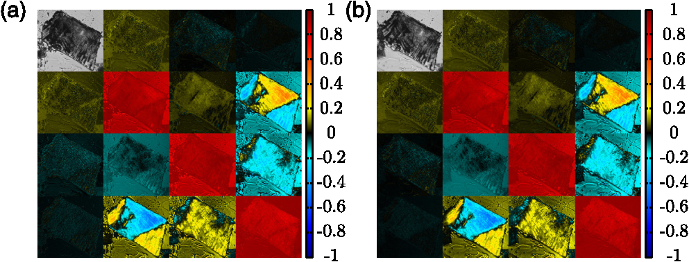

3.1.

Depolarization and Linear Retardance

Linear retardance describes how much the polarization in one direction is phase shifted with respect to its orthogonal polarization. Figure 5 shows the linear retardance together with its uncertainty for the tendon sample. The uncertainty is calculated from $L_u$ and represents the standard deviations of the linear retardance. As previously reported,¹¹ a high concentration of collagen results in a high retardance, mainly due to the form birefringence induced by the shape of the fibers in the effective medium. The mentioned study looked at the collagen fibers present in cartilage, which is less ordered than the collagen fibers in tendons. Being less ordered means that the structure should be modeled as a multilayered effective medium (requiring a layered decomposition of the Mueller matrix) with one orientation for every layer. The higher degree of order in the tendon makes the presented results more clear, and thus avoids the need to consider the sample as a multilayered system.

Fig. 5

Linear retardance (a) and the uncertainty (b) for the tendon sample at normal incidence. Both images are in degrees.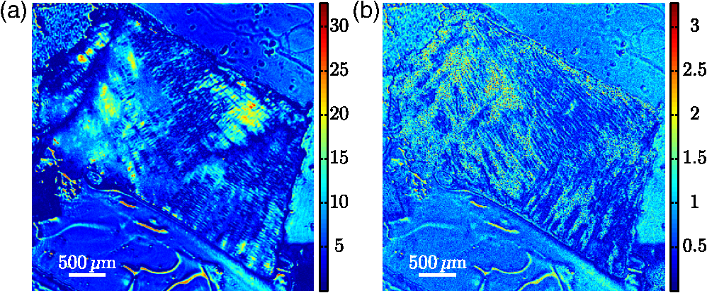

Figure 5(b) shows the uncertainty image (standard deviation) of the linear retardance, which is seen to be above the random noise level in some areas. As the uncertainty in this figure is a result of depolarization effects, it is useful for the analysis of the sample. Previous evaluation of the uncertainty has been limited to the knowledge of the measurement error found from the calibration. Specifically, the error is found from the measurement of air which, here, results in a measurement error on the order of a few percents. The uncertainty image supplies additional information about the sample. It gives a measure for the uncertainty induced by randomness in the sample. This randomness can, for instance, be the fiber orientations and/or sizes, as well as depolarizing effects like multiple scattering and integration over several polarization states in one pixel. This is confirmed by comparing the uncertainty measurement to the depolarization shown in Fig. 6(a).

Fig. 6

(a) Depolarization at normal incidence for the tendon sample. The color scale is from 0 for fully polarized to 1 for fully depolarized. (b) Uncertainty in the direction of the slow axis for normal incidence. The color scale is in degrees.

3.2.

Directional Imaging

From the retardance found in the decomposition, it is not only possible to calculate the linear retardance, but also the direction of the fast axis of the birefringence. This latter property can, together with the correct effective medium model, be used to find the direction of the collagen fibers as explained in Sec. 2.

The directional image and the SHG image for the tendon sample are shown in Fig. 7. As the 3-D directional image in Fig. 7(a) shows, the fibers are mostly in the plane, as expected due to the direction of the cryostat cut. The calculated in-plane directions [black lines in Figs. 7(a) and 7(b)] correspond very well with the apparent directions in the SHG images [Figs. 7(c) and 7(e)]. There are some areas that are clearly out-of-plane [red areas in the 3-D directional image, Fig. 7(a)], which in the SHG images are either dark or show some weak structure. The latter can be explained by the SHG signal generation. When considering SHG signal generation, fiber orientations are important, as a fiber in-plane has a much larger cross section for generating SHG, compared to one out-of-plane. This means that the darker parts of the image in Fig. 7(c) probably are due to an out-of-plane orientation of the fibers, in accordance with the 3-D directional image. Figure 7(d) shows an overlay of the out-of-plane part of Fig. 7(a) and the SHG image in Fig. 7(c).

Fig. 7

3-D directional image (a) with a zoomed view (b), an SHG image (c) with a zoomed in view (e) and an overlay of the SHG and the out-of-plane direction of the tendon (d). The colorwheel beside the directional image shows the out-of-plane direction in degrees, with 0 deg being in the image plane and $\pm 90\mathrm{deg}$ normal to the image plane. $+90\mathrm{deg}$ is the direction toward the reader (positive ${\mathrm{\Delta }}^{\log -M}$). The overlay (d) (area outside of the sample masked for clarity) shows the SHG and out-of-plane directions overlain. The yellow color represent the negative out-of-plane direction and the cyan the positive direction. No color represents an in-plane direction and increasing color more out-of-plane.

The lower right of the sample shows an offset between the directional image and the SHG. There could be several reasons for this offset, one being that the size of the fibers is around the upper limit of the validity of the effective medium model, which is $\sim \lambda$ (here $\lambda =940\mathrm{nm}$). In this study, it was necessary that the fibers were sufficiently large to visualize with SHG, which is limited by the diffraction limit. It is expected that the MMI results will be superior for smaller fibers.

Another contributing factor to the error in the direction is the depolarization induced uncertainties in the direction of the fast axis. The calculation of this uncertainty was not given by Kumar et al.¹² as it cannot be calculated from $L_u$ in the same way as the uncertainty in the other parameters. As a solution to this, we have calculated the uncertainty, shown in Fig. 6(b), using the standard method for propagation of errors, here, the uncertainties found in $L_u$. If the propagation is made at an incidence angle of 0 deg, the resulting uncertainty in the angle of the fast axis is given by

The reasons for choosing to study the uncertainty at an incidence angle of 0 deg, instead of $\pm 30\mathrm{deg}$, are due to the approximations used to derive the propagation uncertainty. Propagation of uncertainties uses only the first derivatives and not the higher orders, which for Eq. (4) might be an incorrect approximation. The uncertainty at 0 and $\pm 30\mathrm{deg}$ is expected to be similar, although the exact relation is hard to predict. A prediction is hard because there could be a reduction in the uncertainty as a result of the increase in the number of data points (two data sets), although the increase in apparent thickness could on the other hand increase the uncertainty. As a consequence, the 0 deg uncertainty will be used as a good indication for the $\pm 30\mathrm{deg}$ uncertainty.

By studying Fig. 6(b), it is possible to see that the uncertainty in the directions is larger in the lower right part of the sample compared to the upper, which is in accordance with the comparison between the 3-D image and the SHG image, shown in Fig. 7. In addition, by comparing with Fig. 6(a), it is seen that they correlate well showing that the uncertainty is a result of the depolarization. As the depolarization is generated by, among others, the randomness of the fiber orientations, it offers a better understanding of the sample structure.

The out-of-plane directions in Fig. 7 are seen to correspond well with the same areas in the SHG image. Additionally, by studying Fig. 7(a) and the zoomed in views in Figs. 7(b) and 7(e), it is possible to see that the oscillating structure (the oscillation between green and blue) along the fibers is visible both in the SHG image and the out-of-plane direction image. Both of these results confirm that the 3-D directional imaging finds the correct directions.

It is worth noting that the method described above makes it possible to find the fiber directions using MMI, even though the resolution in our system is much poorer than for SHG. Another notable property is that this method only requires the sample to be birefringent, as the calculation is based on the direction of linear retardance. Linear retardance is present in a range of different biologicals,⁹ colloidals,²⁷ and solid matter systems,²³ extending the possible applications for the method.