On the use of the Cramér–Rao lower bound for diffuse optical imaging system design

Vivian E. Pera; Dana H. Brooks; Mark J. Niedre

doi:10.1117/1.JBO.19.2.025002

6 February 2014 On the use of the Cramér–Rao lower bound for diffuse optical imaging system design

Vivian E. Pera, Dana H. Brooks, Mark J. Niedre

Author Affiliations +

Journal of Biomedical Optics, Vol. 19, Issue 2, 025002 (February 2014). https://doi.org/10.1117/1.JBO.19.2.025002

Abstract

We evaluated the potential of the Cramér–Rao lower bound (CRLB) to serve as a design metric for diffuse optical imaging systems. The CRLB defines the best achievable precision of any estimator for a given data model; it is often used in the statistical signal processing community for feasibility studies and system design. Computing the CRLB requires inverting the Fisher information matrix (FIM), however, which is usually ill-conditioned (and often underdetermined) in the case of diffuse optical tomography (DOT). We regularized the FIM by assuming that the inhomogeneity to be imaged was a point target and assessed the ability of point-target CRLBs to predict system performance in a typical DOT setting in silico. Our reconstructions, obtained with a common iterative algebraic technique, revealed that these bounds are not good predictors of imaging performance across different system configurations, even in a relative sense. This study demonstrates that agreement between the trends predicted by the CRLBs and imaging performance obtained with reconstruction algorithms that rely on a different regularization approach cannot be assumed a priori. Moreover, it underscores the importance of taking into account the intended regularization method when attempting to optimize source–detector configurations.

1. Introduction

A persistent topic in diffuse optical imaging has been how best to design source and detector configurations. Although it is always possible to simulate data with different source-detector configurations and evaluate the image reconstruction results according to various metrics (e.g., bias and variance,¹ mutual information²), doing so can be very time- and resource-intensive. For these reasons, there has been enduring interest in methods that allow one to optimize the design of these configurations without having to repeatedly solve the inverse problem. One such approach that has proven popular is singular value analysis (SVA), which involves computing the singular value spectrum of the Jacobian (sensitivity matrix of the forward problem) associated with a particular system configuration and counting the number of singular values above a given threshold.³^–⁹ While SVA is conceptually straightforward, it does not make use of the information contained in the singular vectors of the Jacobian, which can lead to errors in performance predictions.¹⁰^,¹¹ It also does not exploit knowledge of the covariance of the measurements. In part to address these shortcomings, some have proposed using the Cramér–Rao lower bound (CRLB) as an alternative design guide.¹²^–¹⁴ The CRLB defines the best achievable precision of any estimator for a given data model and has long been used in the statistical signal processing community—especially in the radar and sonar signal processing communities—to perform feasibility studies and system design. Like SVA, computing the CRLB does not require solving the inverse problem and should therefore be independent of the method selected to do this in practice. But unlike SVA, which can give only a relative indication of system performance overall, the CRLB can in principle yield numerical values of precision as a function of parameters of interest (e.g., inhomogeneity depth). Although other metrics have been recently proposed to optimize the design of data collection strategies for diffuse optical (DOT)¹⁵ and fluorescence-mediated tomography (FMT),¹⁶ to our knowledge only the CRLB can potentially provide the significant advantage of quantitative estimates of performance. We note that despite yielding a lower bound on theoretically available precision, the CRLB does not guarantee that any particular image reconstruction algorithm will be able to reach or even approach the bound. However, in many settings, including the diffuse optical imaging work cited above, differences in the CRLB are used as a surrogate measure of potential reconstruction accuracy. Thus, to be useful for system design, the CRLB should predict performance trends of reasonable reconstruction algorithms as imaging configurations vary.

Obtaining the CRLB requires inverting the Fisher information matrix (FIM), however, which is usually ill-conditioned (and often underdetermined) in the case of DOT and FMT. Here, we consider the impact of regularizing the FIM (so that it may be inverted) on the ability of so-computed CRLBs to predict system performance in a typical DOT setting. To the best of our knowledge, this issue has not been previously addressed in the diffuse optical imaging community. As we discuss in Sec. 2.1, one way of regularizing the FIM is to assume that the inhomogeneity to be imaged is a point target—an approach that initially appears reasonable since this is often a first step in the analysis of more complex problems (i.e., analogous to using the point spread function (PSF) to characterize instrument performance in optical microscopy). In what follows, we probe the often unexamined assumption that the CRLBs computed for a point target are good predictors of imaging performance obtained with traditional image reconstruction algorithms. We illustrate that the utility of the CRLB for ill-posed problems such as DOT is limited, even under ideal conditions, and that a proper interpretation of the results requires taking into account the methods used to regularize the FIM and the inverse problem.

This article is organized as follows: in Sec. 2, we discuss the computation of the CRLB and the challenge that an ill-conditioned FIM matrix presents. We review two types of strategies to cope with this challenge and further explore the point-target approach with simulations. The results of our investigation are presented in Sec. 3, and we conclude in Sec. 4 with a discussion of the implications for the utility of the CRLB in diffuse optical imaging system design and the importance of considering the regularization method.

2. Methods

2.1.

CRLB for the Linearized DOT Problem: General Target

The CRLB considered here defines the lowest variance that any unbiased estimator can achieve assuming a given probabilistic data model.¹⁷ The basic idea is that the curvature of the log-likelihood function of the data model determines the accuracy with which a particular unknown (e.g., position of an inhomogeneity) may be estimated. Log-likelihood functions that are sharply peaked about the unknown quantity permit a more accurate estimate of its value, while the reverse is true for log-likelihood functions that are rather flat in the neighborhood of the unknown. The CRLB provides a measure of this curvature. It is computed for a vector of unknowns by first calculating the FIM, which consists of second derivatives (and first derivative cross products) of the log-likelihood function with respect to each unknown, and then taking its inverse.

Consider the linearized DOT inverse problem for the case of an absorbing inhomogeneity with differential absorbance distribution $δ μ_{a}$ and data model

Eq. (1)

y = b + J δ μ_{a} + n,

where

y

denotes a vector of independent source-detector measurements,

b

contains the known background values in the absence of the inhomogeneity,

J

is the Jacobian or sensitivity matrix, and

n

represents the additive Poisson noise associated with each measurement. (Vector and matrix quantities appear here in bold font.) The CRLB for estimating the values of the differential absorbance over the imaging domain (i.e., the elements of the vector

δ μ_{a}

) is given by

Eq. (2)

C (δ μ_{a}) = {(J^{T} R^{- 1} J)}^{- 1},

where

{[*]}^{T}

denotes the transpose, and

R

is a diagonal covariance matrix containing the mean of the measurements on its diagonal (i.e.,

{[R]}_{j j} = {[b + J δ μ_{a}]}_{j}

). This result is obtained by a simple modification of the derivation in Ref. 18 to account for a nonzero background signal. The matrix

J^{T} R^{- 1} J

is the FIM and is at best ill-conditioned (if not low rank) in the case of diffuse optical imaging. An ill-conditioned FIM signifies in this case that our data alone do not contain sufficient information to extract all of the unknown values that we desire from it in a numerically stable manner.

Two approaches for overcoming this roadblock to computing the CRLB have been adopted in the literature. The first regularizes the FIM by adding to it a regularization matrix as is common in, for example, Tikhonov regularization.¹² However, because this regularized FIM has not been derived directly from the data model, it is technically no longer a CRLB. One might assume that it is possible to limit the amount of regularization applied so that the bounds computed from this “perturbed” FIM are in reasonable agreement with the true CRLBs. This is an assumption that to our knowledge has not been investigated in the context of ill-posed problems like diffuse optical imaging. We note that in some cases, it might be possible to associate a regularized FIM with an appropriate data model. For example, if a Bayesian perspective is adopted with a white noise Gaussian distribution serving as the prior for $δ μ_{a}$ , then the resulting FIM will have the same structure as a Tikhonov-regularized matrix. The inverse of this matrix is known as the Bayesian CRLB.¹⁹ Such a data model, however, is not always useful; for example, it is known to produce overly smooth solutions at the expense of image resolution. Moreover, in the scenarios reported here, we found it impossible to choose a physically meaningful regularization parameter for this model that did not dominate the resulting CRLB estimate, thus making the latter essentially a reflection of assumed prior knowledge.

The second approach regularizes the FIM by reparameterizing the problem, which results in a reduction of the number of unknowns to be estimated from the data. Approaches that consider the inhomogeneity to be a point target¹³^,²⁰ or a target with a constant $δ μ_{a}$ and an easily parameterized geometric form (e.g., a sphere)¹⁴ fall into this category. When such an assumption is appropriate and this information is used to solve the inverse problem, a maximum likelihood (ML) algorithm can usually attain the CRLBs, resulting in performance that is typically at least an order of magnitude better than what can be achieved with standard reconstruction approaches.²¹ Unfortunately, data models with a reduced number of unknowns can usually only model a limited subset of scenarios of interest.

It is certainly the case, however, that the resolution of an optical imaging system is often characterized by its ability to image a point target.²² Moreover, using a point target as a proxy for a more complex object is ubiquitous in science. In what follows, we investigate whether CRLBs computed for the case of a point target can be used to predict performance trends when standard DOT reconstruction algorithms (that do not make use of the point-target assumption) are used to solve the inverse problem. Without making use of all of the information available (i.e., that the inhomogeneity is a point target), it is unlikely that any unbiased algorithm will approach the CRLBs, so the resulting numerical estimates of precision will probably not be meaningful per se. But we consider here to what degree they might be useful as relative measures of performance amongst different system configurations as a function of parameters of interest (e.g., inhomogeneity location, $δ μ_{a}$ , etc.).

2.2.

CRLB for the Linearized DOT Problem: Point Target

To compute the CRLB for a point target, we re-write $δ μ_{a}$ as the product of a scalar $δ μ_{a}$ and a unit vector $e_{i}$ , which contains zeros everywhere except for the $i$ ’th component which is equal to 1. This component encodes the location of the point target in the imaging domain. Our vector of unknowns is $ϕ = [r, θ, δ μ_{a}]$ , where $(r, θ)$ denotes the position of the point target and $δ μ_{a}$ its differential absorbance. We use polar coordinates for position here, since we consider a circular imaging geometry in Sec. 2.3 [see Fig. 1(a)]. The resulting CRLB given the Poisson noise model specified by Eq. (1) is

Eq. (3)

C (ϕ_{i}) = {[\begin{matrix} δ μ_{a}^{T} {\dot{J}}_{r}^{T} R^{- 1} {\dot{J}}_{r} δ μ_{a} & δ μ_{a}^{T} {\dot{J}}_{r}^{T} R^{- 1} {\dot{J}}_{θ} δ μ_{a} & e_{i}^{T} J^{T} R^{- 1} {\dot{J}}_{r} δ μ_{a} \\ δ μ_{a}^{T} {\dot{J}}_{r}^{T} R^{- 1} {\dot{J}}_{θ} δ μ_{a} & δ μ_{a}^{T} {\dot{J}}_{θ}^{T} R^{- 1} {\dot{J}}_{θ} δ μ_{a} & e_{i}^{T} J^{T} R^{- 1} {\dot{J}}_{θ} δ μ_{a} \\ e_{i}^{T} J^{T} R^{- 1} {\dot{J}}_{r} δ μ_{a} & e_{i}^{T} J^{T} R^{- 1} {\dot{J}}_{θ} δ μ_{a} & e_{i}^{T} J^{T} R^{- 1} {Je}_{i} \end{matrix}]}^{- 1},

where

ϕ_{i}

denotes the vector of unknowns associated with a point target at location specified by

e_{i}

,

{\dot{J}}_{r} = \partial J / \partial r

, and

{\dot{J}}_{θ} = \partial J / \partial θ

. The diagonal components of the matrix

C (ϕ_{i})

represent the lower bounds on the variance of the target’s radial position, angle, and

δ μ_{a}

estimates (i.e.,

σ^{2} (r) \geq {[C (ϕ_{i})]}_{11}

,

σ^{2} (θ) \geq {[C (ϕ_{i})]}_{22}

, and

σ^{2} (δ μ_{a}) \geq {[C (ϕ_{i})]}_{33}

).

Fig. 1

(a) Schematic of four source-detector configurations considered; configurations rotate about the sample obtaining measurements every 5 deg. Positions of source and detectors are denoted by “s” and “d,” respectively; angular positions of detectors are listed in brackets. Point-target Cramér–Rao lower bounds (CRLBs) for (b) target radial position and (c) $δ μ_{a}$ as a function of target depth.

2.3.

Point-target DOT Simulations

We considered a continuous-wave DOT system with a transmissive circular imaging geometry, although a similar investigation could be carried out for other imaging geometries and modalities (e.g., FMT) with minor modifications to Eq. (3). As shown in Fig. 1(a), we modeled four source-detector configurations that rotate about a 25-mm diameter sample obtaining measurements every 5 deg. This resulted in a total of $3 \times 72 = 216$ measurements for the sparsest configuration (det3), and $37 \times 72 = 2664$ for the densest (det37). The source, detectors, and absorbing inhomogeneity (point target) were assumed to lie in the same plane. We employed the diffusion approximation to the Boltzmann transport equation for an infinite homogeneous medium to compute $J$ , assuming background optical properties of $μ_{a} = 0.02 {mm}^{- 1}$ and $μ_{s}^{'} = 1.5 {mm}^{- 1}$ typical of those encountered in small animal imaging.²³ The assumption of an infinite homogeneous medium allowed us to rely on analytical forms for the Green’s functions that comprise $J$ , which permitted us to side-step the potential complication of computing derivatives of $J$ numerically in Eq. (3).

The (noise-free) forward data was modeled as

Eq. (4)

y_{0} (r_{di}, r_{s}) = β G^{C W} (r_{di}, r_{s}) + δ μ_{a} J e_{i},

where

y_{0}

is an

M \times 1

vector of measurements for each source-detector pair, with

r_{di}

and

r_{s}

representing the locations of the

i

’th detector and source, respectively;

M

is the total number of measurements;

β

is a scale factor that determines the signal-to-noise ratio (SNR); and

G^{C W} (r_{di}, r_{s})

is an

M \times 1

vector of continuous-wave Green’s functions for a three-dimensional infinite homogeneous scattering medium. The product

J e_{i}

forms an

M \times 1

vector with each component equal to

- β G^{C W} (r_{di}, r) G^{C W} (r, r_{s}) Δ v

, where

r

represents the location of the point target (encoded by

e_{i}

), and

Δ v

is the volume of a voxel in the reconstruction grid. The value of

δ μ_{a}

was set to

2 {mm}^{- 1}

to produce sufficient contrast so that the target could be easily reconstructed. Although this is

100 \times

the background value, we have explicitly defined our data model as linear (after background subtraction) in Eq. (4), so the use of the linear image reconstruction algorithm described in the following paragraph is appropriate. We scaled the maximum value obtained from each source-detector configuration when no absorbing inhomogeneity was present to

10^{4}

counts, which could be considered the equivalent of adjusting the source power so as to avoid saturating any detector in a particular configuration. We then added Poisson noise to the modeled data, yielding measurements with 1% to 4% noise. Fifty realizations of measurements for each configuration for an embedded point target at various depths (

r = 1

, 4, 7, and 10 mm) were generated. We used a grid size of 0.25-mm pixels to compute the forward data, which effectively placed a lower limit on the size of the point target, but all two-dimensional reconstructions were performed with a coarser Jacobian (0.5-mm pixels) to avoid inverse crimes.

To perform the image reconstructions, we used a common algebraic iterative technique, the randomized Kaczmarz method (also known as r-ART) implemented in Ref. 24. We employed a relaxation parameter of 1.5 along with a non-negativity constraint and used 50 iterations per reconstruction. These parameters were selected to yield stable results of acceptable quality for all source-detector configurations.

3. Results

3.1.

Cramér–Rao Lower Bounds

The CRLBs computed for a point target as a function of target radial position or depth are displayed in Figs. 1(b) and 1(c). Figure 1(b) illustrates the CRLBs for target depth, while Fig. 1(c) displays the CRLBs for target $δ μ_{a}$ . The bounds for target angle as a function of target radial position are not shown; they are essentially uniform for each detector configuration, except in the immediate vicinity of $r = 0$ where angle is not uniquely defined. (Because we collect measurements over a full 360 deg, the CRLBs show no dependency on target angle, so results as a function of target angle are also not shown for brevity.) Since the bounds are reported as standard deviations, lower values indicate better (i.e., more accurate) performance. We see that as expected, all detector configurations perform better with a shallow target than a more deeply embedded one. From these plots, with respect to estimating target depth, we expect the nine-detector configuration that goes out to $\pm 45 \deg$ (det9_45) to perform about as well as the 37-detector configuration (det37), which has more than four times the number of measurements. Surprisingly, the other nine-detector configuration (det9_90) is similar in performance to the three-detector configuration (det3). With respect to estimating target $δ μ_{a}$ , performance as a function of depth is rather stable, although the configurations with detectors at $\pm 90 \deg$ (det9_90 and det37) seem to suffer when the target is deeper. We note that the trends observed in these plots are in part a direct result of the way that we have chosen to limit the maximum SNR for each configuration, as detectors closer to 0 deg in configurations with elements at $\pm 90 \deg$ , see SNRs that are lower than than what they measure in the $\pm 35$ or $\pm 45 \deg$ configurations. If we did not equalize the the maximum SNR across configurations, those with detectors at $\pm 90 \deg$ would have the advantage, since being closer to the source, these detectors would measure higher SNRs. In general, however, given our manner of capping SNR per configuration, those detector arrangements without elements that go out to $\pm 90 degrees$ appear to have a distinct performance advantage.

3.2.

Reconstructions

Example reconstructions with the randomized Kaczmarz method (which does not assume a point target) from the four detector configurations for a deep ( $r = 4 mm$ ) and shallow ( $r = 10 mm$ ) target are displayed in Fig. 2. In Tables 1 and 2, we summarize the reconstruction results of the 50 realizations per configuration using a number of metrics. (Although we have chosen to focus on the results for $r = 4 mm$ and $r = 10 mm$ as exemplars of a deep and shallow target, respectively, similar conclusions can be drawn from the data at $r = 1 mm$ and $r = 7 mm$ , which is not shown for brevity.) In Table 1, we compare the standard deviation of the radial position estimate (columns 4 and 5), defined as the location of the peak value of each reconstruction, with the CRLBs (columns 2 and 3) for the deep and shallow targets. We display normalized values in columns 3 and 4 to make comparing relative performance easier. We also include the bias and the average full-width half-maximum (FWHM) area of the reconstructed spots. We show similar metrics in Table 2 for the $δ μ_{a}$ estimate, which is defined as the peak value of each reconstruction. In Table 2, we notice that the precision estimates for $δ μ_{a}$ computed from the reconstructions are lower than the CRLBs. This is not an inconsistency, since we see from column 6 that the $δ μ_{a}$ estimates are significantly biased, so in this case, we would not expect lower bounds computed for unbiased estimates to apply. Overall, we see a lack of correspondence between columns 3 and 4 in both tables, which represent the normalized predicted (from the CRLBs) and computed (from the reconstructions) values for the precision of target radial position and $δ μ_{a}$ estimates. We also note that no single measure seems to be able to capture imaging performance for a point target. For example, although the reconstructed position estimate for the shallow target with det37 has the smallest bias, the standard deviation for this detector configuration is larger than that of det9_45, which has a larger bias but a standard deviation of 0.

Fig. 2

Sample reconstructions for deep target ( $r = 4 mm$ , upper row) and shallow target ( $r = 10 mm$ , bottom row).

Table 1

Target radial position estimate: Cramér–Rao lower bound (CRLB) and reconstruction results. Sigma (σ) denotes the standard deviation. Results for deep target (r=4 mm) are in upper half; shallow target (r=10 mm) in lower half. Normalized σ(r) results (columns 3 and 4) were obtained from σ(r) (columns 2 and 5) by dividing by the maximum σ(r) value (deep and shallow targets considered separately). Bias is the average reconstruction position estimate minus the true value; the FWHM denotes the average area enclosed by the half-max contour.

Deep/Shallow	CRLB		Reconstruction
Deep/Shallow	$σ (r)$ (mm)	Normalized $σ (r)$	Normalized $σ (r)$	$σ (r)$ (mm)	Bias (mm)	FWHM ( ${mm}^{2}$ )
det3	0.080	1.00	1.00	0.21	1.39	16.68
det9_45	0.050	0.63	0.57	0.12	0.97	9.00
det9_90	0.080	1.00	0.97	0.20	$- 0.07$	9.73
det37	0.042	0.53	0.00	0.00	0.00	4.02
det3	0.030	1.00	1.00	0.32	1.87	8.77
det9_45	0.019	0.64	0.00	0.00	0.50	6.63
det9_90	0.026	0.90	0.22	0.07	0.49	4.79
det37	0.014	0.47	0.55	0.18	0.43	2.93

Table 2

Target δμa estimate: CRLB and reconstruction results. Sigma (σ) denotes the standard deviation. Results for deep target (r=4 mm) are in upper half; shallow target (r=10 mm) in lower half. Normalized σ(δμa) results (columns 3 and 4) were obtained from σ(δμa) (columns 2 and 5) by dividing by the maximum σ(δμa) value (deep and shallow targets considered separately). Bias is the average reconstruction δμa estimate minus the true value.

Deep/Shallow	CRLB		Reconstruction
Deep/Shallow	$σ (δ μ_{a})$ ( ${mm}^{- 1}$ )	Normalized $σ (δ μ_{a})$	Normalized $σ (δ μ_{a})$	$σ (δ μ_{a})$ ( ${mm}^{- 1}$ )	Bias ( ${mm}^{- 1}$ )
det3	0.015	0.51	0.66	0.0011	$- 1.98$
det9_45	0.010	0.33	0.88	0.0014	$- 1.96$
det9_90	0.030	1.00	0.83	0.0014	$- 1.96$
det37	0.015	0.51	1.00	0.0016	$- 1.92$
det3	0.016	1.00	0.54	0.0041	$- 1.96$
det9_45	0.010	0.64	0.36	0.0027	$- 1.94$
det9_90	0.015	0.95	0.66	0.0049	$- 1.91$
det37	0.008	0.49	1.00	0.0075	$- 1.84$

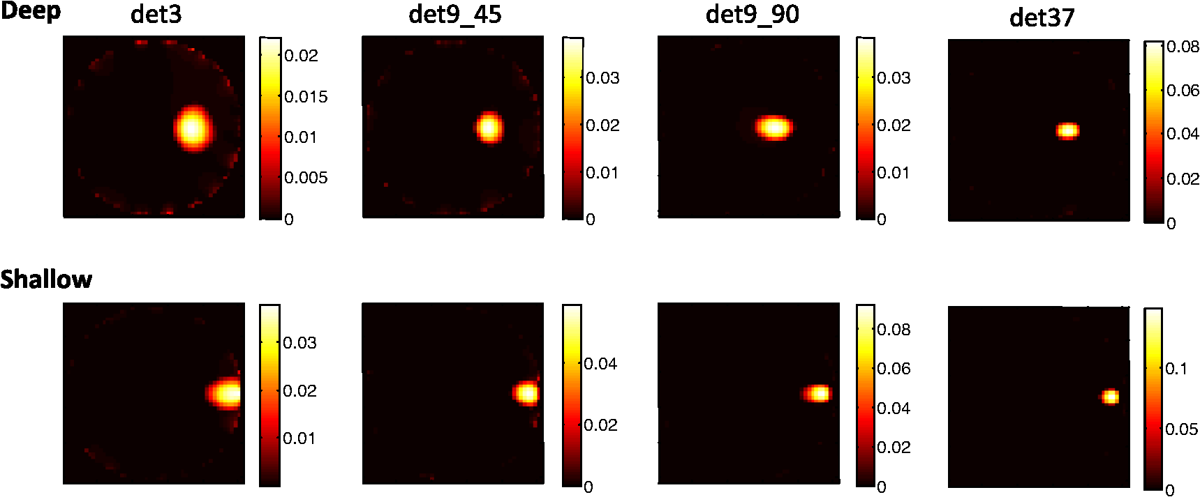
Within the three-detector configuration (det3), we did find a correspondence between the average FWHM area and the CRLB for the precision of target radial position as a function of depth, as shown in Fig. 3(a). Such a relationship did not hold up, however, when comparing different detector configurations for the same target depths, as seen in Table 1, nor was it as strong in other source-detector configurations [e.g., det37 in Fig. 3(b)].

Fig. 3

Comparison of normalized FWHM area from reconstructions to normalized CRLB for target depth for (a) three-detector configuration and (b) 37-detector configuration. The FWHM areas (symbols) and CRLB (curve) were each normalized separately by dividing by their maximum value. Standard errors for the FWHM values are similar in magnitude to the symbol size and are therefore not shown.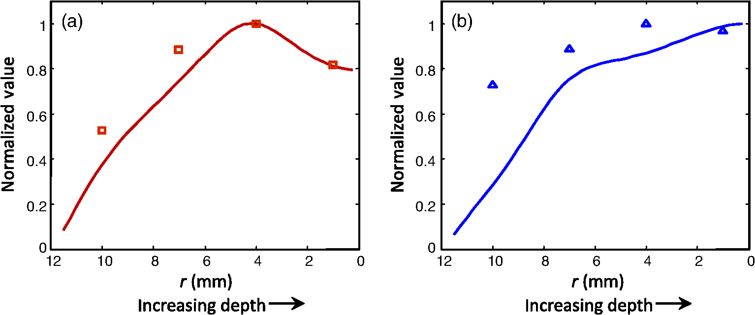

4. Discussion and Conclusions

In this work, we evaluated the potential of the CRLB to serve as a design metric for diffuse optical imaging systems. In the case of DOT and FMT, computing the CRLB requires inverting a matrix that is usually ill-conditioned (if not rank deficient), so a decision about how to regularize the problem must be made before the bound can be determined. Our choice to regularize by employing a point-target model was motivated by the fact that imaging systems are frequently characterized by their ability to resolve point targets (e.g., the imaging PSF), and the approach had been previously reported in the literature.¹³ We reiterate that we did not expect to obtain imaging performance that quantitatively approached the CRLBs, since we relied on a common inversion algorithm (randomized Kaczmarz method) that did not make use of the point-target assumption. Rather, we tested the hypothesis that point-target CRLBs could be used to predict relative instrument performance. Although we did see some relative agreement between the FWHM values and the CRLB for radial position as a function of target depth, overall our results indicate that point-target CRLBs are not good predictors of imaging performance across different system configurations when standard reconstruction algorithms are employed. This is likely because the impact of regularization across the different system configurations varies depending on the regularization method, e.g., point-target assumption or randomized Kaczmarz method. The agreement seen within a detector configuration suggests that both of these methods share a similar sensitivity to target depth. Although an examination of the effects of the different regularization schemes on the CRLB might shed further light on our results, this represents a substantial analysis in its own right and is beyond the scope of the present paper. We point out that because our investigation was conducted in silico, there were no unmodeled sources of error present aside from the coarser Jacobian used in the reconstructions. That the point-target CRLBs did not prove useful in this situation calls into question their predictive value under more realistic circumstances (e.g., when the inhomogeneity is not a point target).

The point-target CRLBs as computed here are for unbiased estimators, and since one of the consequences of regularization is the introduction of bias in order to stabilize the solution of an ill-posed inverse problem, one might wonder why these bounds would apply to the case of diffuse optical imaging in the first place. Although some have argued that DOT reconstructions are unbiased in the limit of sufficient iterations and high SNR¹² or a large number of source–detector pairs,¹⁴ this is certainly a valid objection in our case, as our reconstructions do exhibit notable bias in the $δ μ_{a}$ estimate. But incorporating bias into the CRLB calculation often requires information that in practice is not usually available, so this does not appear to be a useful alternative.

It is also the case that the CRLB represents the best achievable performance for a given data model and therefore not necessarily the expected performance with a particular algorithm. To check whether our results would hold up using a different reconstruction algorithm, we modeled and reconstructed the same data using NIRFAST²⁵ (results not shown), an FEM-based package for modeling light transport in tissue that uses a modified Tikhonov regularization scheme to perform image reconstruction. This also did not produce trends that agreed with the point-target CRLBs. Since we only considered two image reconstruction algorithms here, our results do not preclude the possibility of obtaining agreement with the CRLBs using a different algorithm and/or imaging geometry or modality, as others have reported.¹²^,¹⁴ But they do establish that such agreement cannot be assumed a priori when the method of regularizing the inverse solution (e.g., iterative algebraic or modified Tikhonov approaches) does not match the one used to compute the CRLBs (e.g., point-target assumption). From a Bayesian perspective, this outcome is not surprising, since according to this view, a different way of regularizing the inverse solution corresponds to a different data model, and CRLBs are specific to the data model assumed. Of course, a CRLB that applies only to estimators that employ a particular regularization strategy is certainly less powerful and useful than one that applies to the class of all unbiased estimators. Moreover, it is not clear how the regularizing effect of iterative techniques like the randomized Kaczmarz method or modified Tikhonov approach (with a regularization parameter that depends on the iteration number) could be incorporated into the CRLB calculation. Progress in this area could expand the range of reconstruction algorithms for which appropriate CRLBs might be determined.

Despite these issues, the CRLB can be successfully employed in diffuse optical imaging if the regularization of the FIM and inverse problem are properly considered. For example, in Ref. 21, we used point-target CRLBs to characterize the performance of a ML estimator designed to localize a single fluorescently-labeled cell in the field of view—effectively a point target given the reconstruction grid. For this application, point-target CRLBs can be employed to optimize the source-detector configuration, since the ML estimator used in the reconstruction relies on the point-target assumption. In Ref. 26, regularization was achieved by reparameterizing the problem using a spherical harmonic basis, which reduced the number of unknowns to be estimated from the data to an object center position and various shape parameters. The CRLB for the shape parameters was subsequently computed and used to provide confidence limits for the shape estimates. The important caveat in both of these cases is that the FIM was regularized by an assumption appropriate to the problem wherein the CRLB was to be employed.

The larger question that our study raises is whether it is possible, even in principle, to optimize the design of an imaging system independently of the regularization scheme when regularization is an integral part of image formation. If our goal had been to image a point target using a reconstruction algorithm that made use of this assumption (e.g., an ML approach, as in Ref. 21, capable of achieving the CRLBs), the det9_45 configuration would offer us performance as good as or better than any of the other source-detector configurations considered here [see Figs. 1(b) and 1(c)]. But, if we rely on more common image reconstruction algorithms like the randomized Kaczmarz method or the modified Tikhonov approach, then our simulations demonstrate that in this case, the det37 configuration delivers markedly improved performance (see Fig. 2 and Tables 1 and 2). Given the necessity of regularization in diffuse optical imaging and the strong impact it can have on results, our study argues for the importance of taking this aspect of image formation into consideration when attempting to optimize source–detector configurations.

Acknowledgments

We thank Christ Richmond of MIT Lincoln Laboratory for insightful discussions on the topic of Cramér-Rao bounds. This work was funded by a grant from the National Institutes of Health (R01EB012117).

References

1.

B. W. Pogueet al., “Statistical analysis of nonlinearly reconstructed near-infrared tomographic images: Part I-theory and simulations,” IEEE Trans. Med. Imag., 21 (7), 755 –763 (2002). http://dx.doi.org/10.1109/TMI.2002.801155 ITMID4 0278-0062 Google Scholar

2.

A. B. Milsteinet al., “Fluorescence optical diffusion tomography using multiple-frequency data,” J. Opt. Soc. Am. A, 21 (6), 1035 –1049 (2004). http://dx.doi.org/10.1364/JOSAA.21.001035 JOAOD6 0740-3232 Google Scholar

3.

J. P. Culveret al., “Optimization of optode arrangements for diffuse optical tomography: a singular value analysis,” Opt. Lett., 26 (10), 701 –703 (2001). http://dx.doi.org/10.1364/OL.26.000701 OPLEDP 0146-9592 Google Scholar

4.

H. Xuet al., “Near-infrared imaging in the small animal brain: optimization of fiber positions,” J. Biomed. Opt., 8 (1), 102 –110 (2003). http://dx.doi.org/10.1117/1.1528597 JBOPFO 1083-3668 Google Scholar

5.

E. E. Graveset al., “Singular-value analysis and optimization of experimental parameters in fluorescence molecular tomography,” J. Opt. Soc. Am. A, 21 (2), 231 –241 (2004). http://dx.doi.org/10.1364/JOSAA.21.000231 JOAOD6 0740-3232 Google Scholar

6.

T. LasserV. Ntziachristos, “Optimization of 360 degrees projection fluorescence molecular tomography,” Med. Image Anal., 11 (4), 389 –399 (2007). Google Scholar

7.

X. ZhangC. Badea, “Effects of sampling strategy on image quality in noncontact panoramic fluorescence diffuse optical tomography for small animal imaging,” Opt. Express, 17 (7), 5125 –5138 (2009). http://dx.doi.org/10.1364/OE.17.005125 OPEXFF 1094-4087 Google Scholar

8.

F. Leblondet al., “Early-photon fluorescence tomography: spatial resolution improvements and noise stability considerations,” J. Opt. Soc. Am. A, 26 (6), 1444 –1457 (2009). http://dx.doi.org/10.1364/JOSAA.26.001444 JOAOD6 0740-3232 Google Scholar

9.

D. Wanget al., “Full-angle fluorescence diffuse optical tomography with spatially coded parallel excitation,” IEEE Trans. Inf. Tech. Biomed., 14 (6), 1346 –1354 (2010). http://dx.doi.org/10.1109/TITB.2010.2077306 ITIBFX 1089-7771 Google Scholar

10.

A. J. Chaudhariet al., “Hyperspectral and multispectral bioluminescence optical tomography for small animal imaging,” Phys. Med. Biol., 50 (23), 5421 –5441 (2005). http://dx.doi.org/10.1088/0031-9155/50/23/001 PHMBA7 0031-9155 Google Scholar

11.

F. LeblondK. M. TichauerB. W. Pogue, “Singular value decomposition metrics show limitations of detector design in diffuse fluorescence tomography,” Biomed. Opt. Express, 1 (5), 1514 –1531 (2010). http://dx.doi.org/10.1364/BOE.1.001514 BOEICL 2156-7085 Google Scholar

12.

P. K. Yalavarthyet al., “Cramér-Rao estimation of error limits for diffuse optical tomography with spatial prior information,” Proc. SPIE, 6434 643403 (2007). http://dx.doi.org/10.1117/12.699404 PSISDG 0277-786X Google Scholar

13.

M. Boffetyet al., “Cramer-Rao analysis of steady-state and time-domain fluorescence diffuse optical imaging,” Biomed. Opt. Express, 2 (6), 1626 –1636 (2011). http://dx.doi.org/10.1364/BOE.2.001626 BOEICL 2156-7085 Google Scholar

14.

L. ChenN. Chen, “Optimization of source and detector configurations based on Cramer-Rao lower bound analysis,” J. Biomed. Opt., 16 (3), 035001 (2011). http://dx.doi.org/10.1117/1.3549738 JBOPFO 1083-3668 Google Scholar

15.

D. KarkalaP. K. Yalavarthy, “Data-resolution based optimization of the data-collection strategy for near infrared diffuse optical tomography,” Med. Phys., 39 (8), 4715 –4725 (2012). http://dx.doi.org/10.1118/1.4736820 MPHYA6 0094-2405 Google Scholar

16.

R. W. HoltF. L. LeblondB. W. Pogue, “Methodology to optimize detector geometry in fluorescence tomography of tissue using the minimized curvature of the summed diffuse sensitivity projections,” J. Opt. Soc. Am. A, 30 (8), 1613 –1619 (2013). http://dx.doi.org/10.1364/JOSAA.30.001613 JOAOD6 0740-3232 Google Scholar

17.

S. M. Kay, Fundamentals of Statistical Signal Processing: Estimation Theory, Prentice-Hall, Upper Saddle River, NJ (1993). Google Scholar

18.

M. UnserM. Eden, “Maximum likelihood estimation of linear signal parameters for Poisson processes,” IEEE Trans. Acoust. Speech Signal Process., 36 (6), 942 –945 (1988). http://dx.doi.org/10.1109/29.1613 IETABA 0096-3518 Google Scholar

19.

Van TreesH. L., Detection, Estimation, and Modulation Theory: Part 1, Wiley, New York (1968). Google Scholar

20.

A. B. Milsteinet al., “Statistical approach for detection and localization of a fluorescing mouse tumor in intralipid,” Appl. Opt., 44 (12), 2300 –2310 (2005). http://dx.doi.org/10.1364/AO.44.002300 APOPAI 0003-6935 Google Scholar

21.

V. Peraet al., “Maximum likelihood tomographic reconstruction of extremely sparse solutions in diffuse fluorescence flow cytometry,” Opt. Lett., 38 (13), 2357 –2359 (2013). http://dx.doi.org/10.1364/OL.38.002357 OPLEDP 0146-9592 Google Scholar

22.

B. W. Pogueet al., “Image analysis methods for diffuse optical tomography,” J. Biomed. Opt., 11 (3), 033001 (2006). http://dx.doi.org/10.1117/1.2209908 JBOPFO 1083-3668 Google Scholar

23.

M. J. NiedreG. M. TurnerV. Ntziachristos, “Time-resolved imaging of optical coefficients through murine chest cavities,” J. Biomed. Opt., 11 (6), 064017 (2006). http://dx.doi.org/10.1117/1.2400702 JBOPFO 1083-3668 Google Scholar

24.

P. C. HansenM. Saxild-Hansen, “AIR tools—a MATLAB package of algebraic iterative reconstruction methods,” J. Comput. Appl. Math., 236 2167 –2178 (2012). http://dx.doi.org/10.1016/j.cam.2011.09.039 JCAMDI 0377-0427 Google Scholar

25.

H. Dehghaniet al., “Near infrared optical tomography using NIRFAST: algorithm for numerical model and image reconstruction,” Commun. Numer. Methods Eng., 25 (6), 711 –732 (2008). http://dx.doi.org/10.1002/cnm.1162 Google Scholar

26.

G. Bovermanet al., “Estimation and statistical bounds for three-dimensional polar shapes in diffuse optical tomography,” IEEE Trans. Med. Imag., 27 (6), 752 –765 (2008). http://dx.doi.org/10.1109/TMI.2007.911492 ITMID4 0278-0062 Google Scholar

Biography

Vivian Pera received an AB in physics from Harvard University and an MS in electrical engineering from Tufts University. Before returning to school to pursue a doctoral degree, she worked at MIT Lincoln Laboratory developing adaptive signal processing algorithms for radar and sonar applications. She is currently a PhD candidate in the Dept. of Electrical and Computer Engineering at Northeastern University and a member of the Biomedical Optics Research Laboratory.

Dana H. Brooks is a professor of Electrical and Computer Engineering, Northeastern University, and cofounder of their Biomedical Signal Processing, Imaging, Reasoning, and Learning (B-SPIRAL) group and of the Center for Integrative Biomedical Computing at University of Utah. His research includes application of signal processing to medical and biological imaging.

Mark Niedre received his PhD from the University of Toronto in 2004 and he is currently an assistant professor of Electrical and Computer Engineering at Northeastern University in Boston, Massachusetts.

CC BY: © The Authors. Published by SPIE under a Creative Commons Attribution 4.0 Unported License. Distribution or reproduction of this work in whole or in part requires full attribution of the original publication, including its DOI.

Citation Download Citation

Vivian E. Pera, Dana H. Brooks, and Mark J. Niedre "On the use of the Cramér–Rao lower bound for diffuse optical imaging system design," Journal of Biomedical Optics 19(2), 025002 (6 February 2014). https://doi.org/10.1117/1.JBO.19.2.025002

Published: 6 February 2014

Access the abstract

JOURNAL ARTICLE
8 PAGES

DOWNLOAD PAPER SAVE TO MY LIBRARY

GET CITATION

CITATIONS

Cited by 5 scholarly publications.

Explore citations on Lens.org

KEYWORDS

Imaging systems

Optical design

Diffuse optical imaging

Sensors

Data modeling

Reconstruction algorithms

Target detection

1.

Introduction

2.

Methods

2.1.

CRLB for the Linearized DOT Problem: General Target

Eq. (1)

Eq. (2)

2.2.

CRLB for the Linearized DOT Problem: Point Target

Eq. (3)

Fig. 1

2.3.

Point-target DOT Simulations

Eq. (4)

3.

Results

3.1.

Cramér–Rao Lower Bounds

3.2.

Reconstructions

Fig. 2

Table 1

Table 2

Fig. 3

4.

Discussion and Conclusions

Acknowledgments

References

Biography

Show All Keywords

Keywords/Phrases

Search In:

Publication Years