Extension of the GATE Monte-Carlo simulation package to model bioluminescence and fluorescence imaging

Vesna Cuplov; Irene Buvat; Frederic Pain; Sebastien Jan

doi:10.1117/1.JBO.19.2.026004

12 February 2014 Extension of the GATE Monte-Carlo simulation package to model bioluminescence and fluorescence imaging

Vesna Cuplov, Irene Buvat, Frederic Pain, Sebastien Jan

Author Affiliations +

Journal of Biomedical Optics, Vol. 19, Issue 2, 026004 (February 2014). https://doi.org/10.1117/1.JBO.19.2.026004

Abstract

The Geant4 Application for Emission Tomography (GATE) is an advanced open-source software dedicated to Monte-Carlo (MC) simulations in medical imaging involving photon transportation (Positron emission tomography, single photon emission computed tomography, computed tomography) and in particle therapy. In this work, we extend the GATE to support simulations of optical imaging, such as bioluminescence or fluorescence imaging, and validate it against the MC for multilayered media standard simulation tool for biomedical optics in simple geometries. A full simulation set-up for molecular optical imaging (bioluminescence and fluorescence) is implemented in GATE, and images of the light distribution emitted from a phantom demonstrate the relevance of using GATE for optical imaging simulations.

1. Introduction

Monte-Carlo (MC) simulations play an increasing role in medical imaging techniques involving radiations [positron emission tomography (PET), single photon emission computed tomography (SPECT), and computed tomography (CT)]. For these applications, simulations are used to help design and assess new imaging devices, and to optimize the acquisition and data processing protocols. The Geant4 Application for Emission Tomography (GATE)¹^,² open-source simulation platform, based on the Geant4 toolkit,³^,⁴ has been developed since 2002 by the OpenGATE collaboration ( www.opengatecollaboration.org) and is currently widely used by the research community involved in SPECT and PET molecular imaging. Moreover, recently, the rise of optogenetics has opened the possibility to address and trigger action potentials in specific cells with light.⁵ In these experimental paradigms, it is of a great interest to study the light path and fluence distribution in tissues, as the penetration depth and deposited power per millimeter will determine the spatial extension of cell activation. Yet, only coarse experimental measurements and simplified two-dimensional (2-D) modeling are currently used in this rapidly growing field.⁶ The MC simulations might be a great asset in that context.

In the last decade, optical imaging has become a major modality in the preclinical setting, especially for screening cancerous models in mice. Although the transition from bench to bedside is yet to be achieved in most cases, there is an increasing interest for optical imaging of endogenous or exogenous probes. These techniques are generally noninvasive, low cost and allow for real time study of biological processes through three-dimesnional (3-D) images of the light distribution emitted from the surface of small animals or superficial areas in humans. Optical imaging modalities encompass a rapidly growing range of techniques from cell resolution microscopy to full field noninvasive 3-D tomography.⁷ Preclinical imaging of bioluminescence or fluorescence signals from tagged cancerous cells in mouse models has become a reference technique for rapid screening of molecules with a potential therapeutic impact.⁸^,⁹^,¹⁰

The MC modeling in light transport simulations¹¹ is used to optimize imaging systems¹² and data interpretation, to study the optimal structural and optical properties of nanophosphors,¹³ or to simultaneously image two distinct fluorophores with lifetime contrast.¹⁴ The MC software simulating the photon migration in complex 3-D shapes, such as the tetrahedron-based inhomogeneous MC optical simulator,¹⁵ the molecular optical simulation environment,¹⁶ the mesh-based MC,¹⁷ and the MC for multilayered media (MCML),¹⁸ have been thoroughly described before. As complex geometries were obtained at the expense of heavy calculations, in recent years extensive efforts were targeted at increasing the computational efficiency through parallelization using clusters or graphics processing unit (GPU) calculators.¹⁹^,²⁰ Recently, the GAMOS MC application has been upgraded to model the light transport due to Cerenkov effect.²¹ Yet, there is currently no MC code offering the same flexibility for modeling a wide range of experimental set-up as GATE does for nuclear imaging applications. Given that optical imaging is a matter of photon transportation, we present here an extension of GATE so that it can model optical imaging experiments, such as bioluminescence or fluorescence imaging and validate it against the MCML simulation tool.

The resulting extended version of GATE (GATE V6.2) therefore offers an original platform for bioluminescence and fluorescence imaging, including some unique features that are not currently offered by other codes:

• a user friendly implementation of material and surface properties using the extensible markup language (XML)
• the modeling of optical photon polarization
• the modeling of detector motion such as orbiting
• as well as a number of practical features:
• a large panel of surface properties (roughness, reflection types)
• the management of analytical and/or voxelized phantoms and sources
• a complete description of an experimental setup, including detailed modeling of the detector geometry and signal digitization
• several output formats (root, binary images).

In addition to enabling modeling of bioluminescence and fluorescence, the GATE also supports modeling of light propagation in scintillators or other types of photon detectors.

2. Material and Methods

2.1.

Physics of Optical Photon Transportation in Biological Tissues

To model the transportation of optical photons through biological tissues, the GATE defines a set of parameters for each type of tissue: a refractive index, absorption and scattering lengths ( $L_{a}$ and $L_{s}$ ), which represent the average distance an optical photon can travel in a medium before being absorbed or scattered, and an anisotropy coefficient ( $g$ ), which corresponds to the average cosine of the scattering angle. The inverse of the absorption or scattering length is referred to as the absorption or scattering coefficient ( $μ_{a}$ , $μ_{s}$ ). In inhomogeneous media, reduced scattering coefficients ( $μ_{s}^{'}$ ) that pool $μ_{s}$ and $g$ are frequently used. Absorption and scattering coefficients are defined as follows:

L_{a} = \frac{1}{μ_{a}} and L_{s} = \frac{(1 - g)}{μ_{s}^{'}} .

Physics processes at optical wavelengths currently supported by the GATE software are bulk absorption, Rayleigh scattering, Mie scattering, refraction, and reflection at medium boundaries, and fluorescence.

2.1.1.

Absorption process

The absorption by the bulk makes the optical photon disappear. The GATE user has to define the material absorption length through the ABSLENGTH parameter that is the average distance traveled by the photon before being absorbed by the medium. The absorption length is a function of the optical photon wavelength.

2.1.2.

Scattering processes

In the case of elastic scattering of light of wavelength $λ$ by a small object with a characteristic dimension $L$ , two regimes can be defined: the Rayleigh regime when $L ≪ λ$ and the Mie regime when $L$ is comparable to $λ$ .

Rayleigh scattering process

The Rayleigh scattering differential cross section is proportional to $\cos^{2} (θ)$ where $θ$ is the scattering angle. The new direction of the scattered photon has to be perpendicular to the new polarization of the photon in such a way that the final direction, initial and final polarizations are all in one plane. Rayleigh scattering thus depends on the particle polarization. A photon that is not assigned a polarization at production may not be Rayleigh scattered. The GATE user has to provide the material Rayleigh scattering length through the rayleigh parameter that corresponds to the average distance traveled by a photon before it is Rayleigh scattered in the medium. The scattering length is a function of the optical photon wavelength.

Mie scattering process

The Mie solution to Maxwell’s equations takes the form of an analytical infinite series. A common approximation to this solution is called Henyey–Greenstein.²² The probability density function that describes the angular distribution of light is

p_{HG} (\cos θ; g) = \frac{1}{2} \frac{1 - g^{2}}{{(1 + g^{2} - 2 g \cos θ)}^{3 / 2}},

with

\int_{- 1}^{1} p_{HG} (\cos θ; g) d \cos θ = 1 and \int_{- 1}^{1} p_{HG} (\cos θ; g) \cos θ d \cos θ = g .

$θ$ is the optical photon scattering angle and $g$ is the material anisotropy. Accounting for polarization and momentum is performed using the same approach as for Rayleigh scattering; the new direction of the photon has to be perpendicular to the new polarization of the photon in such a way that the final direction and the initial and final polarizations are all in one plane.

Although the Henyey–Greenstein phase function reproduces the forward peak of Mie scattering reasonably well, it does not correctly describe the backscattering. This can be overcome with the use of the double Henyey–Greenstein function, which is a linear combination of Henyey–Greenstein phase functions:²³

p_{d HG} (\cos θ) = f p (\cos θ; g_{F}) + (1 - f) p (\cos θ; g_{B}),

which depends on a forward anisotropy,

g_{F}

, a backward anisotropy,

g_{B}

and a ratio between the forward and backward angles [

f

is a positive fraction in the range (0, 1)]. Table 1 shows the parameters that have to be defined in GATE to simulate the Mie scattering in a biological tissue.

Table 1

Optical properties of the Mie scattering process.

	Parameter definition
MIEHG	Mie scattering length (i.e., $L_{s}$ )
MIEHG_FORWARD	Material forward anisotropy ( $g_{F}$ )
MIEHG_BACKWARD	Material backward anisotropy ( $g_{B}$ )
MIEHG_FORWARD_RATIO	Ratio between forward and backward angles

2.1.3.

Processes at the interface between two media

When an optical photon arrives at a medium boundary, it can undergo total internal reflection, refraction, or reflection, depending on its wavelength, its angle of incidence, and the refractive indices on both sides of the boundary. Geant4 provides the GATE with a large panel of options to simulate surfaces through a set of parameters. (For a complete description of the Geant4 surfaces, we refer the reader to the Geant4 User’s guide.²⁴) Two surface types are available: dielectric_dielectric, which supports reflection and transmission, and dielectric_metal, which only supports reflection and absorption (i.e., detection). Table 2 lists the variety of surface finishes associated with each surface type. Biological tissues would essentially be simulated as polished or ground surfaces. The other surface types would rather be of interest for simulations of materials such as ceramics or plastics. A frontpainted surface is a surface on which a paint is directly applied. A polishedfrontpainted/groundfrontpainted surface will only reflect as specular spike/Lambertian (see Table 3) or absorb light, without any refraction. A backpaint is a reflector coating (i.e., a few micrometers thick coating away from the volume). The refractive index RINDEX of the backpainted surface (i.e., coat) is defined as part of the volume surface. The reflections inside the coat or refractions back out the coat are simulated with the optical process at boundary. For a polishedbackpainted/groundbackpainted surface, polished/ground refers to the coating which reflects as specular spike/Lambertian. In opaque materials, the refractive index is a complex number: the real part describes the refraction and the imaginary part accounts for absorption. In case of a dielectric_metal surface, the probability of reflection (reflectivity) is specified by the user or calculated from the complex refractive index (realrindex and imaginaryrindex) via the Fresnel equations. In case of a dielectric_dielectric surface, the reflectivity is used to determine whether a photon is absorbed by the surface. The probability of transmission (transmittance) can be set by the user when the medium refractive index is unknown. Finally, the probability of detecting a photon is specified by the efficiency parameter. When a biological tissue surface is not explicitly defined by the user, it is by default simulated as a perfectly smooth surface (i.e., polished). In that case, the only relevant property is the refractive index of the two materials on either side of the interface. Refraction and reflection probabilities are calculated from Snell’s law.

Table 2

List of surface type and finish that are available in GATE.

Surface type	Surface finish
dielectric_dielectric	polished, polishedfrontpainted, polishedbackpainted ground, groundfrontpainted, groundbackpainted
dielectric_metal	polished or ground

Table 3

Light reflection types at the interface between two media, which are available when using GATE. The Lambertian reflection is implicit.

	Parameter definition
SPECULARSPIKECONSTANT	Specular reflection about the average surface normal
SPECULARLOBECONSTANT	Specular reflection about the surface normal of the micro facet
BACKSCATTERCONSTANT	Reflection in the direction the optical photon came from (enhanced on very rough surfaces)

In addition, possible irregularities of the boundary surface can be introduced through the sigmaalpha parameter. As shown in Fig. 1, a ground surface is described as a set of microfacets which are distributed around the average surface normal following a Gaussian distribution with a standard deviation $σ_{α}$ . Table 3 lists the various surface reflection types that can be modeled using GATE. The Lambertian (diffuse) reflection is implicit as the sum of the proportion of specularspikeconstant, specularlobeconstant, backscatterconstant, and Lambertian (i.e., diffuse reflection) is constrained to unity. A specular reflection is a mirror-like reflection, which is present in mirrors, ceramics, aluminium, silver, or fruit skin. A diffuse reflection occurs on surfaces such as plaster, fibers (paper), or polycrystalline materials. The specular reflectance description at the air/tissue interface is important for techniques using reflectance measurements. For example, the performance of imaging systems using a probe in contact with tissues might be impacted by the nature of the surface. Several studies have shown that for diagnosis tools using fibers, the relative angle between fiber and tissue as well as the curvature of tissues are critical parameters.

Fig. 1

Light reflection types available in Geant4 Application for Emission Tomography (GATE) through Geant4: Specular spike (i.e., perfect mirror), specular lobe, and diffuse (Lambertian). A ground surface is composed of micro-facets where $α$ is the angle between a microfacet normal and the average surface normal.

2.2.

Simulation of Optical Photon Fluorescence

One of the most common optical imaging approach is fluorescence spectroscopy. This technique involves a fluorescent molecule (or probe), which is excited by an external source of light and then emits photons at longer wavelengths. When selecting the fluorescent agent for its close affinity with the diseased cells, a region with increased fluorescence emission will represent a diseased tissue. Geant4 already simulates the wavelength shifting (WLS) fibers that are widely used in high energy physics experiments.²⁵ These fibers absorb $λ$ wavelength light and re-emit a $λ^{'} > λ$ wavelength light. The WLS physics process was added to GATE in order to enable the simulation of fluorescence in biological tissues. Fluorescence is a material property, therefore, the GATE users have to provide the fluorophore properties as listed in Table 4. The fluorophore concentration is specified through the definition of the voxelized phantom. The scattering properties of the fluorescence photons are specified using the Mie or Rayleigh scattering physics processes of GATE where the scattering length is given as a function of the wavelength.

Table 4

List of optical properties that define a fluorophore in GATE.

	Parameter definition
WLSABSLENGTH	Fluorophore absorption length
WLSCOMPONENT	Fluorophore emission spectrum
WLSTIMECONSTANT	Fluorophore excitation state lifetime
WLSNUMBEROFPHOTONS	Fluorophore quantum yield

2.3.

Validation

2.3.1.

Validation of GATE versus MCML

The simulation set-up used for validating the model implementation in GATE with respect to the MCML simulation results consisted of a rectangular solid Biomimic (INO, Québec, Canada) ( http://www.ino.ca) optical phantom of surface area of $5 \times 5 {cm}^{2}$ and thickness varying from 0.5 to 2 mm. Solid Biomimic optical phantoms are made of polyurethane, visible and near infra-red absorbing dyes and titanium dioxide scatterers. They mimic the optical properties of human and animal tissues. Figure 2 shows the 530-nm wavelength optical photon unidirectional source emitting perpendicularly to the phantom surface and the position of two detecting surfaces on each side of the phantom. We generated 10,000 optical photons in both MCML and GATE simulations. The optical properties of the phantom were measured at two wavelengths by the manufacturer using the time resolved transmittance technique²⁶^,²⁷ and are given in Table 5. The refractive index of the Biomimic phantom was 1.521 and the anisotropy 0.62. For the validation of GATE versus MCML, we systematically calculated the percentage of absorbed, transmitted, and backscattered optical photons obtained with the Biomimic phantom when varying the phantom thickness in two scenarios: (a) when only optical absorption and scattering processes were enabled; (b) when optical physics processes at boundaries were also included, in addition to optical absorption and scattering processes.

Fig. 2

Simulation set-up used for validating the model implementation in GATE versus Monte-Carlo for multilayered media (MCML). Two detecting surfaces were used to count the number of transmitted and reflected optical photons.

Table 5

Biomimic optical phantom absorption and reduced scattering coefficients for two wavelength values.

Wavelength (nm)	$μ_{a}$ ( ${cm}^{- 1}$ )	$μ_{s}^{'}$ ( ${cm}^{- 1}$ )
530	1.18	8.84
630	1.08	9.54

Biological tissues are not perfectly smooth. Geant4 allows the GATE user to define a more realistic surface roughness with the parameter $σ_{α}$ as described in Sec. 2.1 and Fig. 1. This parameter is not well known for biological tissues. Therefore, we studied the sensitivity of the simulation results, in terms of transmittance, absorbance, and reflectance, as a function of the $σ_{α}$ value.

2.3.2.

Modeling of the optical photon fluorescence

Fluorescence emission spectra measured in the laboratory were used as input fluorescence emission spectra in our simulations. Two fluorophores were considered: Rhodamine B and Fluorescein. As shown on Fig. 3, we simulated a set-up consisting of a rectangular analytical phantom of volume $4 \times 4 \times 4 {cm}^{3}$ filled with a fluorescent material and surrounded by a scattering material, whose properties are given in Table 6. The scattering material refractive index was 1.2 and its anisotropy was 0.6. The simulation code currently uses a linear interpolation to derive the material properties at a particular energy. Yet Geant4 allows other interpolation functions such as polynomial or spline. An excitation point source of 387-nm wavelength is emitted isotropically from the center of the phantom. We recorded the wavelength of all optical photons that exited the phantom. No comparison against real data was performed.

Fig. 3

Simulation set-up used for modeling of the optical photon fluorescence in GATE.

Table 6

Optical properties of the scattering material.

Wavelength (nm)	310	530	629	1240
Mie reduced scattering coefficient $μ_{s}^{'}$ ( ${mm}^{- 1}$ )	0.059	0.125	0.307	0.174
Rayleigh scattering coefficient ( ${mm}^{- 1}$ )	0.106	0.107	0.102	0.102
Absorption coefficient ( ${cm}^{- 1}$ )	0.077	0.077	0.077	0.077

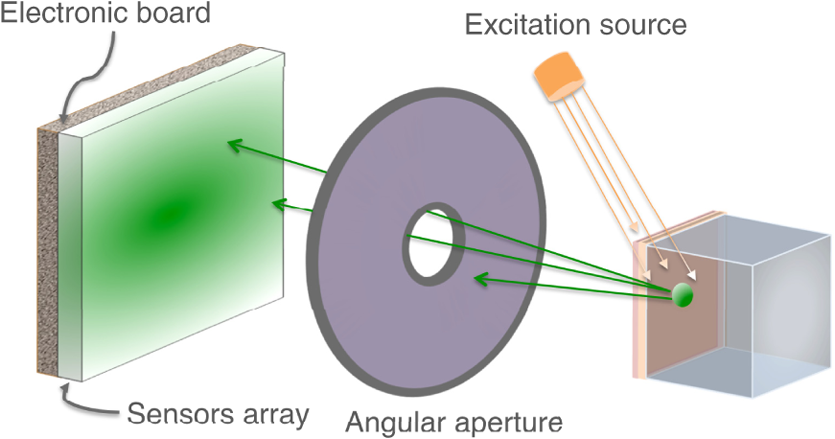
2.4.

Proof of Concept for Optical Imaging Applications

In this section, we show a proof of concept of optical imaging simulations such as bioluminescence and fluorescence imaging. No comparisons against real experiments are performed. Figure 4 shows the optical imaging system and generic phantom used to detect optical photons using GATE in the optical imaging experiments that we simulated. The detector was composed of a $3 \times 3 {cm}^{2}$ array made of $1000 \times 1000 pixels$ of $30 \times 30 - {μ m}^{2}$ area, an electronic board and an angular aperture that limits the range of angles over which the optical system can accept light. The distance between the angular aperture and the detection surface (focal distance) was 5 cm, the diameter of the angular aperture opening was 0.6 cm and the distance between the angular aperture and the phantom was 6 cm. The phantom that we used in our simulations was composed of a $2 \times 2 \times 2 - {cm}^{3}$ box of scattering material and two layers made of either scattering material, hypodermis, or epidermis. The inner layer was 1-mm thick, whereas the outer layer was 0.5-mm thick. Both layers had a surface of $2 \times 2 {cm}^{2}$ . The optical properties of the hypodermis and epidermis in the wavelength range of [560, 665] nm are given in Table 7. The optical properties of the scattering material are given in Table 6.

Fig. 4

Simulated optical imaging detection system and phantom.

Table 7

Optical properties of human hypodermis and epidermis in the wavelength range of [560, 665] nm. These values were taken from Ref. 28.

	$μ_{a}$ ( ${mm}^{- 1}$ )	$μ_{s}^{'}$ ( ${mm}^{- 1}$ )	Anisotropy (g)	Refractive index
Hypodermis	$0.013 \pm 0.005$	$1.26 \pm 0.34$	0.8	1.37
Epidermis	$0.033 \pm 0.009$	$2.73 \pm 0.54$	0.8	1.37

2.4.1.

Bioluminescence simulation

Figure 5 shows the optical imaging system used to detect optical photons when simulating a bioluminescence experiment. The center of a voxelized source (which represents the tumor) of 663-nm wavelength optical photons was positioned at 5 mm under the inner layer of the phantom described in Fig. 4. Each voxel was assigned a specific optical photon flux. Figure 6 shows an axial view of the voxelized source used in our simulations. The size of the tumor along the $x$ , $y$ , and $z$ axes was 6.11, 6.11, and 5.6 mm, respectively. The tumor volume was $0.11 {cm}^{3}$ .

Fig. 5

Simulated bioluminescence experimental set-up.

Fig. 6

Axial slice of the voxelized phantom used in our simulations, which was made of $15 \times 15 \times 9 voxels$ of $0.47 \times 0.47 \times 0.80 {mm}^{3}$ volume.

2.4.2.

Fluorescence simulation

Figure 7 shows the optical imaging system used to detect optical photons in the scenario of a fluorescence experiment. We used a voxelized tumor (same as in Fig. 6) and assigned the Rhodamine B fluorophore, with properties as explained in Sec. 2.3.2, to each voxel of the tumor and positioned it at 5 mm under the inner layer of the phantom described in Fig. 4. The fluorophore was excited by two external beam light sources emitting 561-nm wavelength optical photons toward the tumor. Each beam had a flux of 1000 optical photons per second.

Fig. 7

Simulated fluorescence reflectance imaging set-up: the excitation (illumination) source and the detector were located on the same side of the phantom.

2.4.3.

Bioluminescence simulation in a complex geometry (MOBY)

As shown in Fig. 8, a bioluminescence experiment was simulated using a MOBY²⁹ phantom that contained the following organs: brain, lungs filled with air, kidney, bladder filled with water, and all other organs described as soft tissue (hypodermis). The tumor, described as a voxelized source (same as in Fig. 6), was located at 8 mm below the MOBY phantom surface and emitted optical photons of 663-nm wavelength isotropically. The optical coefficients of the biological tissues used for this simulation are given in Tables 7 and 8. $10^{10}$ optical photons were emitted from the bioluminescence source region.

Fig. 8

Simulated bioluminescence experimental set-up using a complex voxelized phantom (MOBY).

Table 8

Optical properties of human adult brain (gray matter) and kidney at a wavelength of 663 nm. These values were taken from Refs. 30 and 31.

	$μ_{a}$ ( ${cm}^{- 1}$ )	$μ_{s}^{'}$ ( ${cm}^{- 1}$ )	Anisotropy (g)	Refractive index
Brain (gray matter)	0.032	2.64	0.85	1.4
Kidney	0.11	5.15	0.85	1.4

3. Results

3.1.

Validation of GATE versus MCML

For the validation of the physics processes involved in optical photon transportation in biological tissues, we compared the GATE with the MCML software. Figure 9 shows the percentage of absorbed, transmitted, and backscattered optical photons obtained with the Biomimic phantom of different thickness (a) when only optical absorption and scattering processes were enabled; (b) when optical physics processes at boundaries were also included, in addition to optical absorption and scattering processes. Figure 10 shows the number of absorbed, transmitted, and backscattered optical photons obtained with the Biomimic phantom of 1.5-mm thickness defined as a perfectly smooth (i.e., polished) surface and as a rough (i.e., ground) surface associated with a $σ_{α}$ parameter varying from 0 to 21 deg. The horizontal lines in Fig. 10 correspond to the result obtained with MCML, which does not take into account any surface roughness. The GATE can be compared to the MCML result when the surface is defined as polished with a specular spike reflection (a perfectly smooth surface reflects only as specular spike). We considered two scenarios: (a) when the ground surface reflects as 100% specular spike; (b) when the ground surface reflects as a 100% Lambertian (diffuse). The error bars in Fig. 10(a) correspond to statistical uncertainties. In Fig. 10(b) the error bars also include the variation of the simulation results due to the change of seed number in the Mersenne twister³² pseudo random number generator that was used. The GATE physics of optical photon transportation in biological tissues (absorption, Rayleigh and Mie scattering and processes at boundary) is in agreement with the MCML simulation. The $σ_{α}$ parameter (that defines the surface roughness) does not influence much the measurement of the transmittance, absorbance, and reflectance in biological tissues. Therefore, as a first approximation, biological tissues can be simulated as smooth surfaces (i.e., $σ_{α} = 0$ ).

Fig. 9

Number of absorbed, transmitted, and backscattered 530-nm wavelength optical photons obtained for the Biomimic optical phantom target of different thickness. (a) Only optical absorption and scattering processes were enabled and (b) optical physics processes at boundaries were also included.

Fig. 10

Number of absorbed, transmitted, and backscattered 530-nm wavelength optical photons obtained for the Biomimic optical phantom target of 1.5-mm thickness for various $σ_{α}$ values. The horizontal lines correspond to the result obtained with the MCML for a perfectly smooth surface.

3.2.

Validation of the Fluorescence Process

We generated fluorescent photons after exciting a fluorophore (Fluorescein) with a 387-nm wavelength light and tracked them through a scattering material. Figure 11 compares the fluorescent photon wavelength spectrum obtained using GATE in two scenarios: (a) the fluorescent photon is not scattered by a diffuse material; (b) the fluorescent photon is scattered. In absence of absorption and scattering, the emission spectrum of the collected photon spectra was identical to the emission spectra obtained experimentally. This demonstrates that GATE accurately reproduces the well-known Fluorescein emission spectrum.

Fig. 11

Fluorescent photon wavelength spectrum obtained using GATE in two scenarii: (without tracking) the fluorescent photon is not scattered by a diffuse material; (with tracking) the fluorescent photon is scattered.

3.3.

Bioluminescence Simulation

As a proof of concept of a bioluminescence imaging simulation using GATE, Fig. 12 shows the projections in the $X Y$ plane (i.e., detecting surface) of the bioluminescent light emitted from the surface of the phantom described in Fig. 5 in three scenarii: (scenario 1) the two external layers of the phantom are made of a scattering material; (scenario 2) an epidermis layer and a scattering material layer, and (scenario 3) an epidermis layer and an hypodermis layer. In each of these three simulations, we simulated $1.1 \times 10^{10}$ photons in total. The image size corresponds to the detector surface size as described in Sec. 2.4 (i.e., $1000 \times 1000 pixels$ of 0.03-mm size). We also show the profiles (averaged pixel intensity) along the $x$ axis obtained in the region of the image located between the two dashed lines. Table 9 summarizes the profile fit results. The width of the detected bioluminescent light distribution increases with the phantom complexity due to scattering of light in biological tissues.

Fig. 12

Two-dimensional (2-D) images and profiles of the bioluminescence light emitted from the surface of the phantom described in Fig. 5.

Table 9

Bioluminescence experiment profile fit results [mean and full width at half maximum (FWHM)] for the three scenarii from Fig. 12.

Bioluminescence scenario	Mean (mm)	FWHM (mm)
1	$12.00 \pm 0.02$	$3.79 \pm 0.02$
2	$12.14 \pm 0.03$	$4.31 \pm 0.04$
3	$11.94 \pm 0.01$	$11.47 \pm 0.01$

3.4.

Fluorescence Simulation

As a proof of concept of a fluorescence imaging simulation using GATE, Fig. 13 shows the projections in the $X Y$ plane (i.e., detecting surface) of the fluorescent light emitted from the surface of the phantom described in Fig. 7 in three scenarios: (scenario 1) the two external layers of the phantom are made of a scattering material; (scenario 2) an epidermis layer and a scattering material layer and (scenario 3) an epidermis layer and a hypodermis layer. In each of these three simulations, we simulated $1.8 \times 10^{10}$ photons in total. We show the profiles (averaged pixel intensity) along the $x$ axis obtained in the region of the image located between the two dashed lines. Table 10 summarizes the profile fit results. The width of the detected fluorescent light distribution increases with the phantom complexity due to scattering of light in biological tissues. It is also larger than the width of the bioluminescent light distribution because fluorescent photons are emitted isotropically whereas bioluminescent photon trajectory was set in one direction. Figure 14 illustrates a fluorescence experiment using (scenario 1) with a larger statistics: $10^{11}$ optical photons were simulated, among which $6 \times 10^{9}$ underwent a fluorescence process. The Gaussian curve mean value is $11.72 \pm 0.01 mm$ and the full width at half maximum is $12.93 \pm 0.01 mm$ .

Fig. 13

2-D images and profiles of the fluorescence light emitted from the surface of the phantom described in Fig. 7.

Table 10

Fluorescence experiment profile fit results (mean and full width at half maximum) for the three scenarii from Fig. 13.

Fluorescence Scenario	Mean (mm)	FWHM (mm)
1	$11.70 \pm 0.02$	$12.93 \pm 0.02$
2	$11.39 \pm 0.03$	$15.16 \pm 0.04$
3	$11.44 \pm 0.04$	$14.95 \pm 0.04$

Fig. 14

2-D image and profile of the fluorescence experiment using (scenario 1) and a statistic of $10^{11}$ optical photons.

3.5.

Bioluminescence Simulation in a Complex Geometry (MOBY)

Figure 15 represents the 2-D image of the bioluminescent light emitted from the complex voxelized phantom MOBY described in Fig. 8. It also shows the profile along the $x$ axis obtained in the region of the image located between the two dashed lines. We simulated $1.1 \times 10^{10}$ optical photons. The Gaussian curve mean value is $11.73 \pm 0.02 mm$ and the full width at half maximum is $11.36 \pm 0.02 mm$ . Figure 16 shows three projections of the bioluminescent light emitted at the surface of the MOBY phantom. The dashed line emphasizes the contour of the MOBY phantom.

Fig. 15

2-D image and profile of the bioluminescence experiment using a complex voxelized phantom.

Fig. 16

2-D images of the bioluminescence light at the surface of the complex voxelized MOBY phantom.

4. Discussion

We have extended GATE with new features such as the Mie scattering process and the visible light fluorescence so that GATE can now support optical imaging simulations. We validated the optical photon physics processes implemented in GATE by showing an excellent agreement with results produced by the MCML simulation tool. The GATE has significant advantages when compared to the MCML. It can simulate more realistic layer surfaces (i.e., surface roughness) and reflection types for a customized surface, which properties would have been obtained from measurements. It also enables the simulation of a complete experimental set-up including the detector features (geometry and electronic response). In addition, unlike MCML, GATE supports the simulation of complex phantoms (such as the MOBY phantom as illustrated in Sec. 3.5).

In this work, we have demonstrated the flexible use of the GATE to perform a complete simulation of realistic experiments of bioluminescence and fluorescence including modeling of complex heterogeneous biological tissues. The GATE input parameters are introduced through a user-friendly environment (i.e., an XML file), which describes optical properties of materials, surfaces, and fluorophores. Compared to other simulators, the GATE software can simulate any optical imaging experiment (diffuse and ballistic) as each physics process can be enabled separately and the geometrical description of the imaging device is simplified by the well-established list of available volumes inherited from Geant4. The GATE provides different output file formats, including a root tree with a nonexhaustive list of variables and a binary file, which represents the image (projection) that is acquired by the imaging device.

All simulations were performed on a computer with 2 GB RAM processor with 8 cores and a clock speed of 2.7 GHz. Table 11 summarizes the statistics and simulation durations per processor obtained for the simulation of the bioluminescence and fluorescence experiments following the scenarios from Figs. 12 and 13. For the bioluminescence simulation, $5.5 \times 10^{7}$ photons were launched on each of 200 processors, yielding a total of $1.1 \times 10^{10}$ photons. For the fluorescence simulation, $6 \times 10^{7}$ photons were launched on each of 300 processors, yielding a total of $1.8 \times 10^{10}$ photons. For the fluorescence experiment, each simulation of $6 \times 10^{7}$ optical photons resulted in the emission of $3.6 \times 10^{6}$ fluorescent photons.

Table 11

GATE bioluminescence and fluorescence experiment statistics and simulation time duration. All numbers are given per processor.

		Number of simulated photons	CPU duration (s)
Bioluminescence	Scenario 1	$5.5 \times 10^{7}$	4904
	Scenario 2	$5.5 \times 10^{7}$	10805
	Scenario 3	$5.5 \times 10^{7}$	16151
	Complex phantom MOBY	$5.5 \times 10^{7}$	20400
Fluorescence	Scenario 1	$6 \times 10^{7}$	10581
	Scenario 2	$6 \times 10^{7}$	14783
	Scenario 3	$6 \times 10^{7}$	19011

The MC simulations being computationally demanding, we run them on multiprocessors. The GPU now offer a solution to significantly reduce execution times. We developed a proof of concept code specific to the main GATE imaging applications (PET, CT, optical imaging, and the electron ionization effect in radiotherapy) that runs on GPU architecture.³³ This code is currently being integrated within GATE where the voxelized phantom tracking is performed on GPU and the detection on CPU. The acceleration factor due to the photon tracking on GPU was found to be 60 for a PET simulation and 80 for a CT simulation. The development of complete optical imaging simulations using the GPU architecture is in progress.

Optical tomography³⁴ can also be simulated using GATE by rotating (i.e., orbiting) the optical system or by duplicating it along a ring around the patient. The GATE tomographic projections can then be used and combined into an inversion scheme to estimate the sources (e.g., fluorophore dimension and location) that produced the observable image (i.e., fluorescent light distribution). This could be performed using the GATE projections as input of the Time-resolved Optical Absorption and Scattering Tomography (TOAST) software.³⁵ The extended version of GATE can now support a broad range of optical imaging simulations. Yet, the importance of properly setting the numerous parameters needed for an accurate modeling of an experimental set-up should be underlined. Special care should be taken in setting the surface and interface properties of materials and tissues that can significantly impact the output of the simulations.³⁶

5. Conclusion

We have extended the GATE MC simulation tool so that it can now support optical imaging simulations. These new developments were validated against the MCML software. We demonstrated that a bioluminescence or fluorescence experiment could be simulated with GATE using multiprocessors in a reasonable amount of time ( $10^{7}$ optical photons are simulated in an hour). These new features of GATE should make it a valuable tool for investigation of quantitative optical imaging and optical tomography.

Acknowledgments

This work was funded by the French National Research Agency through hGATE project (ANR-09-COSI-004-01). We would like to thank Darine Abi Haidar for providing the measured excitation and emission spectra of Rhodamine B and Fluorescein.

References

1.

Janet al., “GATE: a simulation toolkit for PET and SPECT,” Phys. Med. Biol., 49 4543 –4561 (2004). http://dx.doi.org/10.1088/0031-9155/49/19/007 PHMBA7 0031-9155 Google Scholar

2.

Janet al., “GATE V6: a major enhancement of the GATE simulation platform enabling modeling of CT and radiotherapy,” Phys. Med. Biol., 56 881 –901 (2011). http://dx.doi.org/10.1088/0031-9155/56/4/001 PHMBA7 0031-9155 Google Scholar

3.

“Geant4: A simulation toolkit,” Nucl. Instrum. Methods, A506 250 –303 (2003). NUIMAL 0029-554X Google Scholar

4.

“Geant4 developments and applications,” IEEE Trans. Nucl. Sci., 53 270 –278 (2006). http://dx.doi.org/10.1109/TNS.2006.869826 IETNAE 0018-9499 Google Scholar

5.

E. S. Boydenet al., “Millisecond-timescale, genetically targeted optical control of neural activity,” Nat. Neurosci., 8 1263 –1268 (2005). http://dx.doi.org/10.1038/nn1525 NANEFN 1097-6256 Google Scholar

6.

O. Yizharet al., “Optogenetics in neural systems,” Neuron, 71 (1), 9 –34 (2011). http://dx.doi.org/10.1016/j.neuron.2011.06.004 NERNET 0896-6273 Google Scholar

7.

E. DalimierD. Salomon, “Full-field optical coherence tomography: a new technology for 3D high-resolution skin imaging,” Dermatology, 224 (1), 84 –92 (2012). http://dx.doi.org/10.1159/000337423 DERMEI 0742-3217 Google Scholar

8.

D. S. Kepshireet al., “Imaging of glioma tumor with endogenous fluorescence tomography,” J. Biomed. Opt.J. Biomed. Opt., 1414 (33), 030501039802 (20092009). http://dx.doi.org/10.1117/1.3127202 JBOPFO 1083-3668 Google Scholar

9.

V. Ntziachristos, “Fluorescence molecular imaging,” Ann. Rev. Biomed. Eng., 8 1 –33 (2006). http://dx.doi.org/10.1146/annurev.bioeng.8.061505.095831 ARBEF7 1523-9829 Google Scholar

10.

V. NtziachristosC. BremerR. Weissleder, “Fluorescence imaging with near-infrared light: new technological advances that enable in vivo molecular imaging,” Eur. Radiol., 13 (1), 195 –208 (2003). http://dx.doi.org/10.1007/s00330-002-1524-x EURAE3 1432-1084 Google Scholar

11.

C. G. ZhuQ. Liu, “Review of Monte Carlo modeling of light transport in tissues,” J. Biomed. Opt., 18 (5), 050902 (2013). http://dx.doi.org/10.1117/1.JBO.18.5.050902 JBOPFO 1083-3668 Google Scholar

12.

P. Tianet al., “Monte Carlo simulation of the spatial resolution and depth sensitivity of two-dimensional optical imaging of the brain,” J. Biomed. Opt., 16 (1), 016006 (2011). http://dx.doi.org/10.1117/1.3533263 JBOPFO 1083-3668 Google Scholar

13.

P. F. Liaparinos, “Optical diffusion performance of nanophosphor-based materials for use in medical imaging,” J. Biomed. Opt., 17 (12), 126013 (2012). http://dx.doi.org/10.1117/1.JBO.17.12.126013 JBOPFO 1083-3668 Google Scholar

14.

J. ChenV. VenugopalX. Intes, “Monte Carlo based method for fluorescence tomographic imaging with lifetime multiplexing using time gates,” Biomed. Opt. Express, 2 871 –886 (2011). http://dx.doi.org/10.1364/BOE.2.000871 BOEICL 2156-7085 Google Scholar

15.

H. ShenG. Wang, “A tetrahedron-based inhomogeneous Monte-Carlo optical simulator,” Phys. Med. Biol., 55 947 –962 (2010). http://dx.doi.org/10.1088/0031-9155/55/4/003 PHMBA7 0031-9155 Google Scholar

16.

H. Liet al., “A mouse optical simulation environment to investigate bioluminescent phenomena in the living mouse with the Monte-Carlo method,” Acad. Radiol., 11 (9), 1029 –1038 (2004). http://dx.doi.org/10.1016/j.acra.2004.05.021 1076-6332 Google Scholar

17.

Q. Fang, “Mesh-based Monte-Carlo method using fast ray-tracing in Plücker coordinates,” Biomed. Opt. Express, 1 165 –175 (2010). http://dx.doi.org/10.1364/BOE.1.000165 BOEICL 2156-7085 Google Scholar

18.

L. WangS. L. JacquesL. Zheng, “MCML—Monte-Carlo modeling of light transport in multi-layered tissues,” Comput. Methods Programs Biomed., 47 (2), 131 –146 (1995). http://dx.doi.org/10.1016/0169-2607(95)01640-F CMPBEK 0169-2607 Google Scholar

19.

E. Alerstamet al., “Parallel computing with graphics processing units for high-speed Monte-Carlo simulation of photon migration,” J. Biomed. Opt., 13 (6), 060504 (2008). http://dx.doi.org/10.1117/1.3041496 JBOPFO 1083-3668 Google Scholar

20.

Alerstamet al., “Next-generation acceleration and code optimization for light transport in turbid media using GPUs,” Biomed. Opt. Express, 1 658 –675 (2010). http://dx.doi.org/10.1364/BOE.1.000658 BOEICL 2156-7085 Google Scholar

21.

A. K. Glaser, “A GAMOS plug-in for GEANT4 based Monte Carlo simulation of radiation-induced light transport in biological media,” Biomed. Opt. Express, 4 (5), 741 –759 (2013). http://dx.doi.org/10.1364/BOE.4.000741 BOEICL 2156-7085 Google Scholar

22.

L. G. HenyeyJ. L. Greenstein, “Diffuse radiation in the galaxy,” Astrophys. J., 93 70 –83 (1941). http://dx.doi.org/10.1086/144246 ASJOAB 0004-637X Google Scholar

23.

S. L. JacquesC. A. AlterS. A. Prahl, “Angular dependence of HeNe laser light scattering by human dermis,” Laser Life Sci., 1 309 –333 (1987). LLSCES 0886-0467 Google Scholar

24.

Geant4 Collaboration, (2011) http://www.geant4.web.cern.ch/geant4/UserDocumentation/UsersGuides/ Google Scholar

25.

V. Cavasinniet al., “A method to study light attenuation effects in wavelength shifting fibres,” Nucl. Instrum. Methods, A517 128 –138 (2004). http://dx.doi.org/10.1016/j.nima.2003.09.045 NUIMAL 0029-554X Google Scholar

26.

J. P. Bouchardet al., “Reference optical phantoms for diffuse optical spectroscopy. Part 1—Error analysis of time resolved transmittance characterization method,” Opt. Express, 18 11495 –11507 (2010). http://dx.doi.org/10.1364/OE.18.011495 OPEXFF 1094-4087 Google Scholar

27.

S. L. JacquesB. WangR. Samatham, “Reflectance confocal microscopy of optical phantoms,” Biomed. Opt. Express, 3 (6), 1162 –1172 (2012). http://dx.doi.org/10.1364/BOE.3.001162 BOEICL 2156-7085 Google Scholar

28.

R. Simpsonet al., “Near-Infrared optical properties of ex vivo human skin and subcutaneous tissues measured using the Monte Carlo inversion technique,” Phys. Med. Biol., 43 2465 –2478 (1998). http://dx.doi.org/10.1088/0031-9155/43/9/003 PHMBA7 0031-9155 Google Scholar

29.

W. P. Segarset al., “Development of a 4D digital mouse phantom for molecular imaging research,” Mol. Imaging Biol., 6 (3), 149 –159 (2004). http://dx.doi.org/10.1016/j.mibio.2004.03.002 1536-1632 Google Scholar

30.

T. M. Baranet al., “Optical property measurements establish the feasibility of photodynamic therapy as a minimally invasive intervention for tumors of the kidney,” J. Biomed. Opt., 17 (9), 098002 (2012). http://dx.doi.org/10.1117/1.JBO.17.9.098002 JBOPFO 1083-3668 Google Scholar

31.

P. Rolfe, “In vivo near-infrared spectroscopy,” Annu. Rev. Biomed. Eng., 2 715 –754 (2000). http://dx.doi.org/10.1146/annurev.bioeng.2.1.715 ARBEF7 1523-9829 Google Scholar

32.

M. MatsumotoT. Nishimura, “Mersenne twister: A 623-dimensionally equidistributed uniform pseudorandom number generator,” ACM Trans. Model. Comput. Simul., 8 (1), 3 –30 (1998). http://dx.doi.org/10.1145/272991.272995 ATMCEZ 1049-3301 Google Scholar

33.

J. Bertet al., “Hybrid GATE: A GPU/CPU implementation for imaging and therapy applications,” in IEEE Nucl. Sci. Sympos. Med. Imaging Conf., 2247 –2250 (2012). Google Scholar

34.

S. Arridge, “Optical tomography in medical imaging,” Inverse Probl., 15 41 –93 (1999). http://dx.doi.org/10.1088/0266-5611/15/2/022 INPEEY 0266-5611 Google Scholar

35.

T. Correiaet al., “Split operator method for fluorescence diffuse optical tomography using anisotropic diffusion regularisation with prior anatomical information,” Biomed. Opt. Express, 2 (9), 2632 –2648 (2011). http://dx.doi.org/10.1364/BOE.2.002632 BOEICL 2156-7085 Google Scholar

36.

E. RoncaliS. R. Cherry, “Simulation of light transport in scintillators based on 3D characterization of crystal surfaces,” Phys. Med. Biol., 58 2185 (2013). http://dx.doi.org/10.1088/0031-9155/58/7/2185 PHMBA7 0031-9155 Google Scholar

Biographies of the authors are not available.

Citation Download Citation

Vesna Cuplov, Irene Buvat, Frederic Pain, and Sebastien Jan "Extension of the GATE Monte-Carlo simulation package to model bioluminescence and fluorescence imaging," Journal of Biomedical Optics 19(2), 026004 (12 February 2014). https://doi.org/10.1117/1.JBO.19.2.026004

Published: 12 February 2014

Access the abstract

JOURNAL ARTICLE
13 PAGES

DOWNLOAD PAPER SAVE TO MY LIBRARY

GET CITATION

CITATIONS

Cited by 29 scholarly publications.

Explore citations on Lens.org

RIGHTS & PERMISSIONS

Get copyright permission Get copyright permission on Copyright Marketplace

KEYWORDS

Monte Carlo methods

Luminescence

Scattering

Bioluminescence

Surface finishing

Optical imaging

Tissues

1.

Introduction

2.

Material and Methods

2.1.

Physics of Optical Photon Transportation in Biological Tissues

2.1.1.

Absorption process

2.1.2.

Scattering processes

Rayleigh scattering process

Mie scattering process

Table 1

2.1.3.

Processes at the interface between two media

Table 2

Table 3

Fig. 1

2.2.

Simulation of Optical Photon Fluorescence

Table 4

2.3.

Validation

2.3.1.

Validation of GATE versus MCML

Fig. 2

Table 5

2.3.2.

Modeling of the optical photon fluorescence

Fig. 3

Table 6

2.4.

Proof of Concept for Optical Imaging Applications

Fig. 4

Table 7

2.4.1.

Bioluminescence simulation

Fig. 5

Fig. 6

2.4.2.

Fluorescence simulation

Fig. 7

2.4.3.

Bioluminescence simulation in a complex geometry (MOBY)

Fig. 8

Table 8

3.

Results

3.1.

Validation of GATE versus MCML

Fig. 9

Fig. 10

3.2.

Validation of the Fluorescence Process

Fig. 11

3.3.

Bioluminescence Simulation

Fig. 12

Table 9

3.4.

Fluorescence Simulation

Fig. 13

Table 10

Fig. 14

3.5.

Bioluminescence Simulation in a Complex Geometry (MOBY)

Fig. 15

Fig. 16

4.

Discussion

Table 11

5.

Conclusion

Acknowledgments

References

Show All Keywords

Keywords/Phrases

Search In:

Publication Years