
|
|
1.IntroductionPhotoacoustic [(PA) or optoacoustic] imaging is a technique for visualization of structures with optical absorption contrast in light scattering media. It is based on the excitation of acoustic waves by the thermoelastic effect, when nanosecond duration electromagnetic pulses are absorbed in an object. The distribution of absorbed energy is obtained from broad band ultrasound signals measured outside the object, from which structures with preferential light absorption can be localized. Because of the ability to visualize the interior of optically scattering objects with ultrasound resolution and the good contrast of blood vessels, PA methods have been recognized as a promising imaging tool for biological tissue.1 Depending on the kind of detector, the size of the object, and the reconstruction method various implementations have been developed.1 PA tomography uses small unfocused detectors that receive acoustic signals at many positions around the object. The distribution of absorbed energy density is obtained by applying a tomographic reconstruction algorithm to the signals. PA microscopy techniques, on the other hand, use detectors combined with an acoustic lens to limit the sensitivity of the sensor to a line of sight along the symmetry axis of the lens. Positions of light-absorbing objects along this line can be obtained from the time of flight of the acoustic waves. No tomographic reconstruction is required as the single amplitude scans can be combined to an image plane or volume for two-dimensional (2-D) and three-dimensional (3-D) imaging, respectively. PA sectional imaging can be seen as a combination of the aforementioned methods.2–4 It uses detectors combined with a cylindrical lens to limit the detector sensitivity to a selected plane in an object. After acquisition of signals from many positions around the region of interest, a tomographic reconstruction yields the distribution of absorbed energy within the section. It is possible to stack many such sections to a 3-D PA image. Due to the limited aperture of the cylindrical lens, a 3-D image constructed from a stack of 2-D slices is expected to have inferior resolution in direction perpendicular to the slices compared to a full 3-D tomographic image, where signals are taken from all directions around the object. However, in situations where a defined region of interest within a large object can be covered with several section images, a significant advantage in terms of data acquisition time and computational effort can be achieved compared to full 3-D tomography. This has led to the development of PA tomography arrays, which allow for acquisition of real-time 2-D images from data collected around an object.5,6 Also, with a single detector that rotates around an object, section images can be acquired within a reasonable time owing to the moderate amount of data needed for a 2-D image compared to 3-D imaging.3,4 Moreover, single detector scanning is an easy-to-implement and cost-effective way to create high-resolution PA images. PA section imaging requires acoustic sensors that are equipped with some kind of cylindrical lens. Typical implementations are flat piezoelectric sensors combined with a concave cylindrical acoustic lens or lens less detectors, where the sensor itself has the shape of a cylindrical area.4 Recently, the combination of an optical line sensor with a cylindrical acoustic reflector was also reported.7 For data acquisition, either the sensor is scanned on a circular line around the object or the object is rotated in front of the sensor. Cylindrical lens detectors can be characterized by their focal length, the numerical aperture (NA), and the width in direction of the cylinder axis. These sensor properties determine the quality of the reconstructed image. For instance, it has been demonstrated that the finite width of the sensor gives rise to a progressive deterioration of lateral resolution for points with increasing distance from the center of the circular scanning curve.8 This effect is attributed to the assumption of point-like detectors in the reconstruction, which is based on radial back-projection. Proposed corrections of the blurring employ model-based reconstruction that takes the finite size of the detector into account9,10 or some kind of deconvolution or deblurring method.11 The NA has an effect on the out-of-plane resolution. For the imaging of extended objects, there is a trade-off between out-of-plane resolution and field of view since with a high NA only a narrow region around the rotation axis, to which the sensor is focused, can be imaged with high resolution. The effect of the sensor width on the lateral resolution can be avoided by using an integrating cylindrical detector.4 In the direction of the cylinder axis, this detector is larger than the imaged object. Due to integration of the incoming acoustic waves over this direction, the recorded signals are related to the Radon transform of the initial pressure distribution in the object.12 Applying the inverse Radon transform to the signals leads to a reconstruction without the lateral blur that is seen in reconstructions from finite-width detectors. The difference between point-like, finite-width detectors and integrating detectors is demonstrated in Fig. 1. In a simulation, a PA section image is reconstructed from the center plane of a phantom that consists of nine homogeneously heated spheres with 0.5 mm diameter arranged in three planes, 1 mm apart. A sensor with and a focal length of 20 mm was assumed. A sensor with a width of 5 mm resolves only the sphere lying close to the center of the image. The outer spheres are strongly blurred in lateral direction due to the point detector assumption in the radial back-projection algorithm. By contrast, a detector with 50 mm width creates an image after inverse Radon transform where all objects lying in the plane of interest appear with good lateral resolution. However, this result shows artifacts related to the imperfect focusing properties of the cylindrical lens. These are blurring of objects in radial direction, especially for the outermost sphere at position , and cross-talk from the neighboring planes. Fig. 1Simulated section images from a phantom consisting of nine spherical photoacoustic sources arranged in three planes. (a) Signals are detected with cylindrical sensors having a numerical aperture of and a width of either 5 or 50 mm. (b) Image of the center plane [shaded in (a)] reconstructed by circular back-projection of signals from detector 1. (c) Image reconstructed by inverse Radon transform of signals from detector 2. 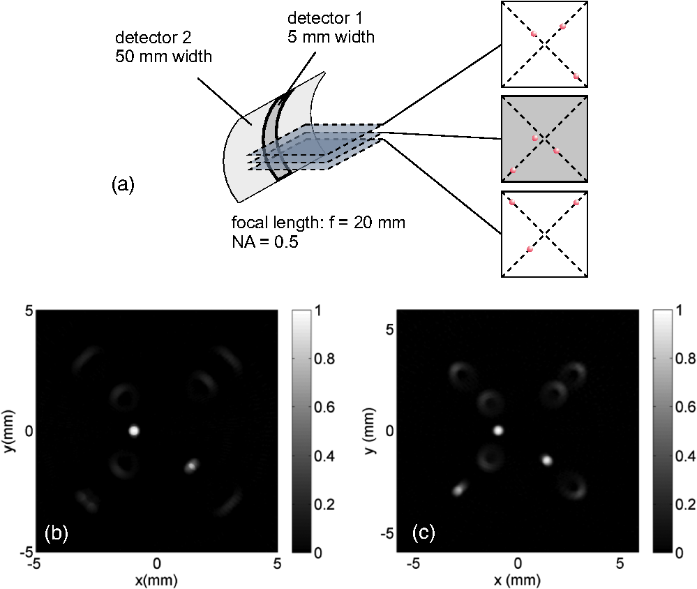 In the present study, we demonstrate how these artifacts can be avoided by employing a model-based, iterative reconstruction algorithm. The aim is to improve the quality of single section images by incorporating information from neighboring sections, rather than a full 3-D imaging technique. For full 3-D imaging, there exist techniques based on unfocused either point-like or line detectors, which yield very good image quality. Our approach is inspired by similar techniques for fluorescence microscopy,13 where the task is to deblur optical sections from out-of-focus light by using information from several section images. In the following, first the model of the forward problem is introduced, followed by the reconstruction algorithm. After outlining the experimental procedures, results from simulations, the experimental verification of the system matrix, and phantom measurements are presented. 2.Methods2.1.Cylindrical Detector ModelFigure 2 shows the cylindrical detector used for this study. The active sensor area has a concave cylindrical shape, determined by its radius of curvature , its width in -direction, and its height in -direction. Its NA is given by . For acquiring a section image, the object is rotated about an axis parallel to the axis. Several sections can be imaged by translating the object or the sensor in -direction. Fig. 2Detector surface for section imaging. The detector is characterized by its radius of curvature , its width in -direction, , and its height in -direction, . The coordinates relative to the detector are and and a point on the detector cross-section is denoted as . To acquire an image, the sample is rotated about an axis parallel to the -direction and is shifted by to cover the entire region of interest. By shifting the object, a target point at moves across the focus plane at . 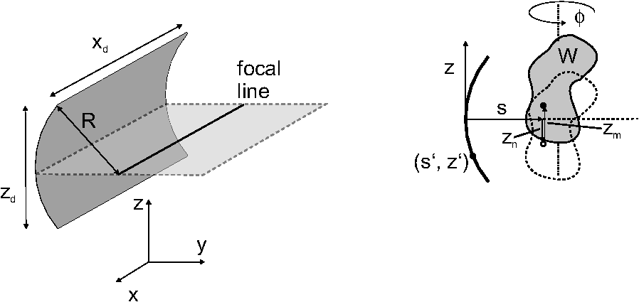 The width exceeds the size of the object to be imaged. To analyze the properties of such an integrating detector, we define a coordinate system relative to the detector and describe its surface as an arrangement of parallel lines, perpendicular to the axis. For a single line oriented along direction, the received signal is the pressure field coming from the object, integrated over the coordinate . Subscript means that the object has been rotated by an angle relative to a reference orientation. Pressure wave is the solution of the acoustic wave equation with as initial condition, where is the Grüneisen parameter and is the absorbed energy density in the rotated object. It can be shown that the integrated pressure signal is a solution of the 2-D wave equation with source ,14 where is a 2-D Radon transform of and is given by Validity of the 2-D solution requires integration limits from minus to plus infinity in Eqs. (1) and (2). It can also be shown, however, that with a finite detector exact integrated signals are measured, provided that the width is sufficiently large.4 For a perfectly focusing detector, the source can be described by and the detector by a single line in the plane at , located at position . Here, we use coordinate , which is the distance between the line detector and a point in the source. It is proportional to the arrival time of the wave emanating from point , where is the speed of sound. The distribution of energy density in a section can then be qualitatively reconstructed by applying the inverse Radon transform to the measured pressure signals.12 However, it has to be taken into account that the pressure signals from a finite source are bipolar, whereas the energy density is purely positive. It is possible to obtain from a quantity that is proportional to the Radon transform of by applying an Abel transform.15 For a single line detector, is proportional to the energy density projected into the plane perpendicular to the line and integrated over a circle with radius around the line position.15 For the focusing detector, which receives signals only from the slice at , the inverse Radon transform of , measured at a sufficient number of angular positions around the imaged slice, directly reconstructs the energy density distribution in this plane.16 Due to the imperfections of the real sensor, contributions from sources outside the focus plane, i.e., at , also have to be taken into account. Furthermore, for sources at , but , the linear dependence between and is not valid. To include all these properties of the real sensor, we describe the forward problem by introducing a system matrix that links the temporal signals measured by the detector to the distribution of absorbed energy density . Since the imaging problem focuses on discrete sections, the -position of the sources is discretized in multiples of , where is the increment between individual sections. For the implementation of the iterative image reconstruction algorithm, a discrete representation of the source distribution is required. We use a representation in uniform spherical expansion functions, as it has been done in similar PA imaging algorithms before.10,17 The resulting system matrix is obtained by calculating the response of the detector to single, homogenously heated spheres residing at grid positions, having a radius on the order of the grid spacing. A response to a single spherical source is calculated by summing the analytical signals received by an infinite line14 over all line positions (typically 200) forming the detector surface. The system matrix is first defined in three dimensions as . It contains the Abel transform and links signals measured at time to sources located at distance in the plane at in the object, which has been shifted in -direction by distance . In our notation, where the sample is rotated and shifted relative to the coordinate system of the sensor, is defined relative to the unshifted sample (dashed contour in Fig. 2). Both and are ranging from to . A signal measured by the cylindrical detector at time , shift position , and angular orientation is denoted by and is related to the 2-D initial energy density distribution by Due to the symmetry of the sensor, the system matrix depends only on . According to the discrete representation of the source distribution , the meaning of is actually the strength of a uniform, spherical voxel located at position in the object rotated by , which is integrated over an infinite line in direction of the cylindrical detector axis. The elements of the system matrix are thus given by where is the response of the detector to a spherical source at position , given byHere, is the analytical signal of a homogenously heated spherical source of radius (on the order of the spatial resolution), located at in the plane offset by from the focus plane of the detector, integrated over a line at position on the detector surface14 (see Fig. 2). Integration over the detector surface is described by the integral of this signal over the curve , the circular arc defining the cross-section of the cylindrical detector surface. The above relation [Eq. (4)] contains one equation for each rotation angle . The system matrix is written here in three dimensions. Alternatively, all recorded signals at one angular orientation can be written as a vector with elements and all sources in another vector with elements . The single layers of (each of them having a different ), denoted by 2-D matrices , can then be arranged in a 2-D matrix with elements , yielding a more convenient way to write this relation. The arrangement of submatrices is 2.2.ReconstructionThe goal of image reconstruction is to find for each projection angle a vector that minimizes the deviation of from the measured signals . Once these values are determined, the final step in image reconstruction is to calculate the source distribution in all recorded sections by applying the inverse Radon transform to . For recovering from , we use the maximum likelihood-expectation maximization (ML-EM) algorithm,18–20 which is known to provide solutions for problems with incomplete or noisy data. It furthermore preserves positivity of the solution, which is important for reconstructing a physically meaningful . The calculation of the iterations requires an adjoint system matrix, which has the effect of a back-projection operator and is the transpose of the real-valued matrix . However, we observed a more rapid convergence of the algorithm by using the following procedure for calculating a modified back-projection operator . In each submatrix , we seek the maximum value of each column and store its index kmax. This gives the most likely arrival time of a wave generated at position in the ’th neighbor plane. “Most likely” in this context means, for instance, that a wave generated by a point source at this position impinges perpendicularly at the sensor surface, giving rise to the maximum detected signal by this source, even if it is not lying on the focal line. Then we build a new matrix as in Eq. (8) that only contains the column wise maxima of . Transposing this matrix yields the back-projection operator with elements , which now links the temporal signals to their most likely source positions. The product then yields a back-projection reconstruction of the data , similar to the focal line concept proposed by Xia et al.21 The iterative reconstruction algorithm for obtaining the ()’th estimate of element of vector is given by To avoid a division by zero, a small scalar on the order of one or two percent of the maximum of is added to the denominator on the right-hand side. This iteration is performed for each rotation angle separately using the temporal signals of all the recorded sections. It has to be taken into account that the projections are not independent of each other since they emanate from the same distribution of absorbed energy. Therefore, at each iteration, the projections are normalized in a way that their integral over distance gives the same value for each section, i.e., for each . This integral can be regarded as a measure of the total energy absorbed in this section and should be equal for all projections. Convergence of the algorithm is monitored by calculating the norm of the residual . After completion of the iterations, the final distribution of the energy density in each of the sections is obtained by applying the inverse Radon transform to the corresponding subsets of . For comparison, we also used an alternative method for the reconstruction of from the measured pressure signals using the lsqr function implemented in MATLAB®. This method, which is suited for large and sparse system matrices, provides a least squares inversion of matrix . 2.3.ExperimentThe model-based reconstruction was tested with a detector made of a 110-μm-thick piezoelectric polyvinylidene fluoride (PVDF) film (Measurement Specialties, Hampton, Virginia) glued onto the concave cylindrical surface of a polyvinyl chloride backing. Detector parameters were a radius of curvature of , a width of , and a height of , giving a numerical aperture of . A thin plastic sheet separated the PVDF film from a water bath, where the sample was placed. Illumination was provided from two sides parallel to the cylinder axis of the detector using pulses from a frequency-doubled, Q-switched Nd:YAG laser (Spectron Laser Systems, Rugby, UK) with a pulse duration of 10 ns. In a first experiment, signals from a small absorber were acquired for comparison with the calculated system matrix. A small, spherical oil droplet with a radius of 150 μm containing black dye was embedded in Agar gel (2% by weight) and was scanned in the -plane perpendicular to the cylinder axis. A range from to (the position of the focal line of the cylindrical detector is at ) and from to was scanned with increments of and . For a tomography experiment, a phantom consisting of clear Agar gel was prepared, containing black oil droplets in two layers apart. During data acquisition, the phantom was scanned to 17 -positions with an increment of 200 μm. At each of the -positions, the phantom was rotated by 360 deg with an angular increment of 1.8 deg. For the reconstruction, the increment in -direction was set to 50 μm. Since it is important to obtain signals from all absorbers at each position of the detector, the phantom was illuminated with a wide beam that covered the whole phantom. In the experiments it turned out that sometimes there remained some negative signal values after the Abel transform. To obtain the purely positive signal necessary for the reconstruction algorithm, the following procedure was used. First, the measured signals were Abel transformed. Then an inverse Radon transform was calculated, yielding a first image of , which contained both positive and unphysical negative components. In this image, the negative parts were set equal to zero, and to the resulting image, the Radon transform was applied. This gave purely positive signals . Compared to simply removing negative values from the Abel-transformed signals, this procedure preserved more of the information content of the data because it avoided the deletion of features residing on negative parts of the signals. 3.Results3.1.SimulationsReconstructions from simulated data are shown in Fig. 3. The same phantom was used as in Fig. 1. Again, the central plane with three spheres is shown. For the calculation, signals from five planes were used: the three planes containing the spherical absorbers and two additional planes at a distance of 1 mm below and above the phantom. Figure 3(a) shows the result of a back-projection, applying the operator to the data, and Fig. 3(b) shows the result after 20 iterations of the ML-EM algorithm in Eq. (9). A reconstruction using 20 iterations of the lsqr algorithm is shown in Fig. 3(c). The back-projection operator leads to a slight improvement of the image quality compared to a direct reconstruction from the Abel-transformed signals [Fig. 1(c)], but only the model-based algorithms are able to eliminate the artifacts. Comparing ML-EM and lsqr methods, both perform similarly in terms of reducing cross-talk and in-plane distortions. The latter, however, yields some residual negative values, as shown in Fig. 3(e). Here, a horizontal profile through one of the sources is displayed together with the reconstruction that is obtained by applying the inverse Radon transform to Abel-transformed pressure signals. No negative values are visible in the profile of the ML-EM reconstruction shown in Fig. 3(d) due to the embedded positivity constraint of this algorithm. The profiles also show a slightly better suppression of cross-talk with the ML-EM algorithm than with the lsqr method. This is seen at position , where the reconstruction from the raw, Abel-transformed signals shows high image values on the order of 0.6. At the same position, the residual peak after lsqr reconstruction reaches a value of , whereas the ML-EM reconstruction yields a negligible value on the order of 0.05. A number of merit for the comparison of the algorithms is the total relative residual, defined as the norm of divided by the norm of . This residual is calculated for the entire measurement data, including all projection angles . Assuming noise-less data as in the shown simulations, the values for the total relative residual are 0.04 for lsqr and 0.11 for ML-EM (both after 20 iterations). Here the lsqr algorithm shows better convergence, although other parameters, such as the reduction of cross-talk, indicate better performance of the ML-EM algorithm. We repeated the simulation with additive Gaussian noise with a standard deviation of 5% of the signal maximum and found relative residuals of 0.30 for lsqr and 0.13 for ML-EM. With these more realistic data the better performance of the ML-EM algorithm in the presence of noise is demonstrated. Fig. 3Simulation results showing section images of the phantom displayed in Fig. 1(a). (a) Applying back-projection operator to the data. (b) Twenty iterations with the maximum likelihood-expectation maximization (ML-EM) algorithm. (c) lsqr reconstruction, all followed by the inverse Radon transform. In (a) to (c) negative values are not displayed. (d) Normalized profiles through the spherical source at , comparing a reconstruction from Abel-transformed raw signals [seen in Fig. 1(c)] with the ML-EM reconstruction. (e) Comparison of profiles through the lsqr reconstruction, again compared to the Abel-transformed raw signals.  3.2.System MatrixExperimental and theoretical signals from a small sphere scanned in the -plane are displayed in Fig. 4. The theoretical signals were obtained by integrating the analytical signals of a sphere with 150 μm radius over the detector surface. In Figs. 4(a) and 4(b) the signals for are shown and in Figs. 4(d) and 4(e) the signals for . In the latter case, the distance between the focus plane and the source was . There is a good agreement between experiment and calculation, showing that the parameters for the simulation of the measurement were properly chosen. This justifies the use of the calculated signal matrix, which was obtained by applying the Abel transform to the columns of the matrix containing the simulated signals. The submatrices with and are displayed in Figs. 4(c) and 4(f). Matrix is close to diagonal with a maximum at the focus, which is located at , and shows some spreading of values at positions outside the focus. Matrix has highest values for -positions outside the focus. Fig. 4Detected signals, system, and back-projection matrices for (upper row) and (lower row). (a) and (d) Experimental signals for a black oil droplet with 0.15 mm radius. (b) and (e) Simulated signals for an absorbing sphere with 0.15 mm radius. (c) System submatrix . (f) System submatrix , both calculated from simulated signals by applying the Abel transform.  3.3.Phantom ExperimentFor image reconstruction, signals from all 17 planes were used, covering the range with the black dye droplets and some extra sections that contained no absorbers. With the spatial increment of 200 μm, the total -range used for reconstruction was 3.2 mm. Reconstructed images in Fig. 5 show one of the sections containing absorbing spherical droplets. Additionally, maximum amplitude projections in -direction reveal the spreading of the imaged objects in direction perpendicular to the sections. A comparison of three reconstruction methods is provided: direct reconstruction applying the inverse Radon transform to Abel-transformed raw data, ML-EM reconstruction, and lsqr inversion. In all images, only positive values are displayed. To quantify the resolution achievable with the different reconstruction methods, Fig. 6(a) compares profiles in -direction through one of the small spheres seen at position , , . This sphere has subresolution size in -direction and is suited for estimating the out-of-plane resolution. In the reconstruction from raw, Abel-transformed pressure signals, the spreading in -direction is largest and amounts to 1.35 mm (FWHM). The two iterative techniques yield better resolution, with 0.86 mm using lsqr and 0.51 mm using ML-EM. Also, a significant improvement of resolution in radial direction becomes evident when plotting the radial intensity profiles of the same sphere, as shown in Fig. 6(b). The radial direction goes through the point (0,0) in the -sections displayed in Figs. 5(a) to 5(c). 4.DiscussionThe goal of this study is to provide artifact-free images from a cylindrical lens detector in PA section imaging. Using the integrating detector concept, where the receiving sensor has a width exceeding the size of the object, it is possible to eliminate the transversal (or tangential) blur that is seen when finite-size detectors are used as an approximation of point detectors. This is a consequence of the relation of the received signals to the Radon transform of the absorbed energy density distribution in the sample. The pressure signal at a given time is an integral of the acoustic pressure field along the direction of the cylindrical lens axis and can be regarded as emanating from a line integral of at distance of from the detector surface. The reconstruction of a slice image from the inverse Radon transform of the Abel-transformed signals still, however, contains artifacts, which can be classified in in-plane distortion and out-of-plane cross-talk. The former is due to the aperture of the cylindrical lens detector, which leads to a limited depth of field. During a full rotation, objects lying in the focus plane at some distance from the rotation axis move in and out of focus, whereas objects near the rotation axis always stay in focus. This description assumes that the rotation axis is located at or near the focal distance, which was the case in our experiments. If a PA source lies at an out-of-focus position, signals from waves emanating at a point in the source are spread over time, leading to a radial blurring in the final image. Cross-talk between sections is due to signals from positions outside the focus plane, which are nevertheless recorded with sufficient strength to create ghost images in the observed section. The two kinds of artifacts are linked because both become worse with distance from the focus. It is not possible to reduce these artifacts by modifications of the imaging hardware. The temporal spreading of signals recorded from out-of-focus sources, which causes the radial blurring, could be reduced by using a smaller NA of the lens, leading to a larger depth of field. However, at the same time, this would enhance cross-talk artifacts owing to the weaker focusing capability of the low-NA lens. For a reduction of cross-talk, the excitation light pulses could be focused into the imaged section, which is usually not possible in strongly light scattering biological tissues. Finally, a large NA means a tight acoustic focus and seems to be able to avoid cross-talk, but only in the narrow region within the focal depth, preventing imaging of extended objects. In the presented experiment, we chose a worst case situation since no optical focusing was applied in sample illumination and at the same time a large NA of 0.5 was chosen for an object that was larger than the depth of field of the lens. Nevertheless, by applying iterative methods, a clear improvement could be obtained compared to the reconstruction from raw data. As in the simulations, both the in-plane distortion and the cross-talk were clearly reduced by applying the model-based reconstruction. Comparing the out-of-plane resolution in Figs. 5 and 6, it appears that the ML-EM reconstruction yields better results than the lsqr method. With the integrating cylindrical detector the reconstruction of several slices can be decomposed into 2-D problems. As first step the reconstruction of each projection separately, which gives a source distribution depending on coordinates and . Due to the integrating property of the sensor, this requires the same system matrix for each projection. Since there is no dependence on the coordinate in direction of the cylinder axis, the corresponding system matrix has a number of elements given by the number of -positions multiplied by the number of temporal samples at all -positions of the detector. The former is given by , the number of positions along , multiplied by the number of sections . The latter is given by the number of temporal samples multiplied again by . The second step of the reconstruction is the inverse 2-D Radon transform, which is applied to each 2-D section separately. The computation of the system matrix for the 17 planes in the phantom experiment (using MATLAB® R2010b on a dual core 2.67 GHz CPU) required 150 s. This time could be reduced by integrating over a smaller number of line elements on the detector surface. We found that already 100 lines gave a sufficiently smooth response. Storage of the submatrices of and required 21 MB of memory. Reconstruction of the phantom required 30 s per iteration of the ML-EM algorithm. For a narrow, nonintegrating detector, the full 3-D problem has to be considered at once. The dependence of detected signals on source position along the cylinder axis has to be taken into account, as well as the number of angles at which signals are taken around the object. This leads to a significantly larger system matrix.9 5.ConclusionImaging of selected slices or sections of an extended object using an acoustic cylindrical lens detector is a cost-effective yet accurate method for PA tomography. The combination of a large, integrating cylindrical lens detector and a model-based reconstruction algorithm leads to a significant reduction of artifacts related to the finite size and imperfect focusing capability of the sensor. Owing to the integrating property of the detector, the reconstruction has to deal with 2-D problems, lowering the computational effort compared to full 3-D reconstruction. Even with a small number of sections, the employed maximum likelihood algorithm yields a significant improvement of image quality compared to direct reconstruction. AcknowledgmentsThis work has been supported by the Austrian Science Fund (FWF), projects S10502 and S10508. ReferencesL. V. WangS. Hu,
“Photoacoustic tomography: in vivo imaging from organelles to organs,”
Science, 335
(6075), 1458
–1462
(2012). http://dx.doi.org/10.1126/science.1216210 SCIEAS 0036-8075 Google Scholar
A. RosenthalV. NtziachristosD. Razansky,
“Model-based optoacoustic inversion with arbitrary-shape detectors,”
Med. Phys., 38
(7), 4285
–4295
(2011). http://dx.doi.org/10.1118/1.3589141 MPHYA6 0094-2405 Google Scholar
R. Maet al.,
“Multispectral optoacoustic tomography (MSOT) scanner for whole-body small animal imaging,”
Opt. Express, 17
(24), 21414
–21426
(2009). http://dx.doi.org/10.1364/OE.17.021414 OPEXFF 1094-4087 Google Scholar
S. Grattet al.,
“Photoacoustic section imaging with an integrating cylindrical detector,”
Biomed. Opt. Express, 2
(11), 2973
–2981
(2011). http://dx.doi.org/10.1364/BOE.2.002973 BOEICL 2156-7085 Google Scholar
A. Taruttiset al.,
“Real-time imaging of cardiovascular dynamics and circulating gold nanorods with multispectral optoacoustic tomography,”
Opt. Express, 18
(19), 19592
–19602
(2010). http://dx.doi.org/10.1364/OE.18.019592 OPEXFF 1094-4087 Google Scholar
J. Gamelinet al.,
“A real-time photoacoustic tomography system for small animals,”
Opt. Express, 17
(13), 10489
–10498
(2009). http://dx.doi.org/10.1364/OE.17.010489 OPEXFF 1094-4087 Google Scholar
R. Nusteret al.,
“Photoacoustic section imaging using an elliptical acoustic mirror and optical detection,”
J. Biomed. Opt., 17
(3), 030503
(2012). http://dx.doi.org/10.1117/1.JBO.17.3.030503 JBOPFO 1083-3668 Google Scholar
M. H. XuL. V. Wang,
“Analytic explanation of spatial resolution related to bandwidth and detector aperture size in thermoacoustic or photoacoustic reconstruction,”
Phys. Rev. E, 67
(5), 056605
(2003). http://dx.doi.org/10.1103/PhysRevE.67.056605 PLEEE8 1063-651X Google Scholar
D. Queiroset al.,
“Modeling the shape of cylindrically focused transducers in three-dimensional optoacoustic tomography,”
J. Biomed. Opt., 18
(7), 076014
(2013). http://dx.doi.org/10.1117/1.JBO.18.7.076014 JBOPFO 1083-3668 Google Scholar
K. Wanget al.,
“An imaging model incorporating ultrasonic transducer properties for three-dimensional optoacoustic tomography,”
IEEE Trans. Med. Imaging, 30
(2), 203
–214
(2011). http://dx.doi.org/10.1109/TMI.2010.2072514 ITMID4 0278-0062 Google Scholar
P. Burgholzeret al.,
“Deconvolution algorithms for photoacoustic tomography to reduce blurring caused by finite sized detectors,”
Proc. SPIE, 8581 858137
(2013). http://dx.doi.org/10.1117/12.2003889 PSISDG 0277-786X Google Scholar
P. Burgholzeret al.,
“Thermoacoustic tomography with integrating area and line detectors,”
IEEE Trans. Ultrason. Ferroelectr. Freq. Control, 52
(9), 1577
–1583
(2005). http://dx.doi.org/10.1109/TUFFC.2005.1516030 ITUCER 0885-3010 Google Scholar
D. A. Agard,
“Optical sectioning microscopy: cellular architecture in three dimensions,”
Ann. Rev. Biophys. Bioeng., 13 191
–219
(1984). http://dx.doi.org/10.1146/annurev.bb.13.060184.001203 ABPBBK 0084-6589 Google Scholar
P. Burgholzeret al.,
“Temporal back-projection algorithms for photoacoustic tomography with integrating line detectors,”
Inverse Probl., 23
(6), 65
–80
(2007). http://dx.doi.org/10.1088/0266-5611/23/6/S06 INPEEY 0266-5611 Google Scholar
G. Paltaufet al.,
“Experimental evaluation of reconstruction algorithms for limited view photoacoustic tomography with line detectors,”
Inverse Probl., 23
(6), S81
–S94
(2007). http://dx.doi.org/10.1088/0266-5611/23/6/S07 INPEEY 0266-5611 Google Scholar
P. ElbauO. ScherzerR. Schulze,
“Reconstruction formulas for photoacoustic sectional imaging,”
Inverse Probl., 28
(4), 045004
(2012). http://dx.doi.org/10.1088/0266-5611/28/4/045004 INPEEY 0266-5611 Google Scholar
P. Ephratet al.,
“Three-dimensional photoacoustic imaging by sparse-array detection and iterative image reconstruction,”
J. Biomed. Opt., 13
(5), 054052
(2008). http://dx.doi.org/10.1117/1.2992131 JBOPFO 1083-3668 Google Scholar
W. H. Richardson,
“Bayesian-based iterative method of image restoration,”
J. Opt. Soc. Am., 62
(1), 55
–59
(1972). http://dx.doi.org/10.1364/JOSA.62.000055 JOSAAH 0030-3941 Google Scholar
L. B. Lucy,
“Iterative technique for rectification of observed distributions,”
Astron. J., 79
(6), 745
–754
(1974). http://dx.doi.org/10.1086/111605 ANJOAA 0004-6256 Google Scholar
M. HaltmeierA. LeitaoE. Resmerita,
“On regularization methods of EM-Kaczmarz type,”
Inverse Probl., 25
(7), 075008
(2009). http://dx.doi.org/10.1088/0266-5611/25/7/075008 INPEEY 0266-5611 Google Scholar
J. Xiaet al.,
“Three-dimensional photoacoustic tomography based on the focal-line concept,”
J. Biomed. Opt., 16
(9), 090505
(2011). http://dx.doi.org/10.1117/1.3625576 JBOPFO 1083-3668 Google Scholar
BiographyGuenther Paltauf received his PhD in physics from the Karl-Franzens-University Graz, Austria, in 1993. After postdoctoral studies in Graz, the University of Bern, Switzerland, and the Oregon Medical Laser Center in Portland, Oregon, he is now associate professor at the Department of Physics at the University of Graz. His research interests are photoacoustic imaging, laser ultrasonics, and photomechanical laser-tissue interactions. Robert Nuster received his PhD in experimental physics from the Karl-Franzens-University Graz, Austria, in 2007 with a thesis on development and application of optical sensors for laser-induced ultrasound detection. From 2008 to 2011, he was a postdoctoral research fellow at the Karl-Franzens-University Graz. Since 2011, he has been a senior postdoctoral research fellow. His current research interests include photoacoustic imaging, characterization of materials by laser ultrasound, and ultrasound sensor development. |


