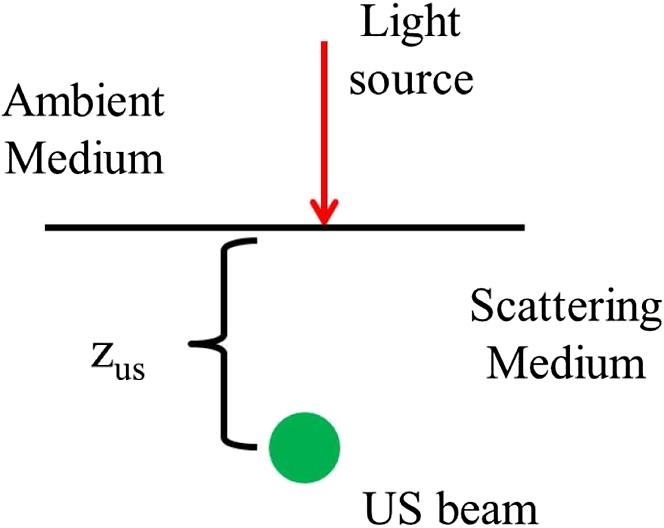
1.

Introduction

Precise measurements of physiological parameters are necessary to increase the accuracy of medical diagnostics, thus reducing unwanted surgical procedures, such as biopsies. Optical methods are well suited for this task, but their resolution degrades quickly with imaging depth because biological tissue is typically highly scattering. For example, confocal microscopy offers a resolution of 1 to 2 μm but is limited to an imaging depth of 100 to 300 μm.¹ Optical coherence tomography is able to increase the imaging depth at the cost of resolution.

However, several techniques combining ultrasound (US) and optical measurements have been developed to increase resolution and imaging depth while maintaining biological sensitivity. One such method mixes a focused US beam with light in tissue to create a diffusive wave modulated at the US frequency, which may then be measured utilizing interferometry, or a system capable of collecting an image at the US frequency.^2–4 Kothapalli et al.⁵ utilized this method with US frequencies up to 75 MHz to experimentally obtain image resolutions in the tens of microns.

Recently, it has been shown that the US-modulated light can be used as a guidestar, and the frequency-shifted wavefront can be utilized to correct for the effects of scattering.^6,7 This technique can achieve US-resolution images at depths of several millimeters.⁷ It has recently been shown that this method can achieve lateral resolutions of 5 μm by the use of initial probe beam wavefront permutation and optimization.⁸

The interaction of light and sound in an optically clear medium has been understood for over 80 years.⁹ However, the interaction is much harder to predict in a scattering medium, such as biological tissue. A model was put forth for US modulation of an optical signal in an infinite homogeneous scattering medium¹⁰ and solved using a Monte Carlo simulation.¹¹ This model was later improved upon for a US plane wave in an arbitrary medium.^12–16 Other work has ignored the coherent effects of light scattering and treats diffuse light using the radiative transport equation (RTE).¹⁷ Recently, Hollmann et al.¹⁸ developed a finite-difference time-domain (FDTD) model that is capable of solving for the modulated field. These simulations all have the disadvantage of being computationally intensive and requiring long run times, although efforts have been made in parallelizing and executing the Monte Carlo code on relatively quick graphical processing units.^19,20

This paper will relate the incident optical flux and fluence rate, and the depth and strength of the US beam, to the resulting diffuse optical signal. We will accomplish this by linking the initial and US-modulated optical field, and develop a relationship for the US-modulated radiance. We will use this to develop a Green’s function for the modulated diffusive wave.

The intent of this paper is to focus on high US frequencies necessary for high-resolution imaging because they are of interest for applications such as phase conjugation. This paper will focus on experimental systems that use frequencies of 45 MHz and above to achieve high-resolution images.^7,8 The results will be validated using an FDTD simulation developed previously.¹⁸ After validating the model, we will use the results to develop a closed-form diffusion equation for the modulated sidebands.

2.

Diffusion

We will review photon transport through a scattering medium and the diffusion approximation to the RTE²¹ in this section. Several authors offer a thorough discussion on this subject.^22–24 However, we will briefly review the salient features here. The fluence rate describes the energy flow per unit area per unit time and is independent of flow direction:

The quantities $L$, $\mathrm{\Phi }$, and $\overrightarrow{J}$ have units of power per area and are fundamentally incoherent. A homogeneous turbid medium is modeled as having a scattering coefficient (${\mu }_s$) that quantifies the scatterer’s cross-sectional area per unit volume. The medium also has an absorption coefficient (${\mu }_a$), which similarly describes the absorber’s cross-sectional area per unit volume. The scattering anisotropy ($g$) is the average cosine of the scattered field resulting from a plane wave interacting with a single scatterer. However, the diffusion equation requires scattering to be isotropic, so an equivalent reduced, or transport, scattering coefficient is given by ${\mu }_s^{\prime }={\mu }_s(1-g)$. A transport mean-free path describes the length after which a light ray loses memory of its incoming direction and is given as ${\ell }_t^{\prime }={({\mu }_s^{\prime }+{\mu }_a)}^{-1}$.

The radiance and source term may be expanded using spherical harmonics. Truncating the expansion after the second-term results in the $P_1$ approximation to the RTE, or

Solving the RTE with this approximation in a turbid medium leads to the diffusion equation

The source term from the RTE is expanded in a similar manner and results in a monopole and dipole term. The monopole is given as

The underlined terms may be ignored.²² Using this simplification, the fluence rate may be written in terms of a differential equation:

Another simplification occurs by assuming the scalar and vector sources are viewed at a large enough distance that they appear to be a single isotropic point source. The new point source is, therefore, given an offset in the direction of the flux.^22,25 The approximations utilized to derive the diffusion equation limit its region of validity to distances greater than one ${\ell }_t^{\prime }$ away from the source.

Typical applications utilizing the diffusion equation include a boundary between the turbid medium and a nonscattering medium, such as air or water. This interface is normally accounted for by using the extrapolated boundary conditions, which stipulate there is an equal but opposite point source located on the opposite side of the boundary that forces the fluence rate to be zero at some distance above the interface.²³ Furthermore, the extrapolated boundary conditions utilize scale factors for the fluence rate and flux to account for any index of refraction mismatch. Solving for these scale factors can be complicated, but tables and linear models of these coefficients exist elsewhere.^26,27

3.

US Modulation

This section will relate the field of the probe beam to the radiance of the US-modulated diffusive wave. The modulated field will then be related to the fluence and flux of the diffusive wave. We will then use this relationship to create the monopole and dipole sources discussed in the previous section.

A focused US beam with an angular frequency, ${\omega }_{\mathrm{us}}$, will interact with the optical signal by linearly modulating the local index of refraction and introduce a phase delay in the probe field. Although there is a potential for other US–optical interactions through the displacement or deformation of scattering particles, these effects are assumed to be minimal at high frequencies. This is because it has been shown that the importance of the index of refraction modulation grows exponentially larger than particle displacement with decreasing US wavelength.¹⁰ Likewise, nonlinear effects, such as particle motion due to radiation pressure and heating, may also exist, but these effects do not produce modulation at the US frequency. This US model is similar to previously published US–optical simulations.¹⁸

3.2.

Field-Radiance Relationship

This section reviews the relationship between the field and the radiance. This will allow us to use the results in Sec. 3.1 to relate the probe beam field to the radiance modulated at $f_{\mathrm{us}}$. To accomplish this, we first decompose the electric field in an infinitesimally small area into a series of angle-dependent plane waves, as shown in Fig. 1. Each angular-dependent plane wave has the form

Eq. (15)

$$F(\widehat{\mathrm{\Omega }})=A(\widehat{\mathrm{\Omega }})e^{j{\omega }_{o}t},$$

where $A(\widehat{\mathrm{\Omega }})$ is the complex amplitude of the field. The field is described by the coherent combination of $F$ over all $\widehat{\mathrm{\Omega }}$.

Eq. (16)

$$E=\iint F(\widehat{\mathrm{\Omega }}){\mathrm{d}}^2\widehat{\mathrm{\Omega }}.$$

Fig. 1

The field in an infinitesimally small volume is decomposed into a series of angle-dependent plane waves, 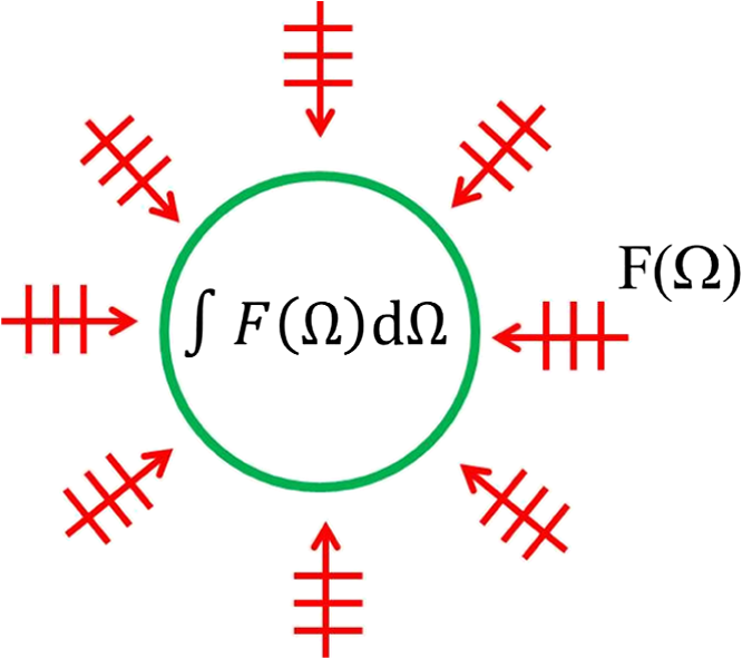$F(\widehat{\mathrm{\Omega }})$.

In a scattering medium, $F(\widehat{\mathrm{\Omega }})$ is uncorrelated so that

Eq. (17)

$$\langle F(\widehat{\mathrm{\Omega }})F^{*}({\widehat{\mathrm{\Omega }}}^{\prime })\rangle =0,$$

for $\widehat{\mathrm{\Omega }}\ne {\widehat{\mathrm{\Omega }}}^{\prime }$. The brackets, $\langle \rangle$, refer to the expected value of the field term. In Monte Carlo the expectation operation is handled by randomly varying the scatterers in the medium during the simulation.²⁸ The decomposition of the electric field may be related to the incoherent irradiance:

Eq. (18)

$$\begin{gathered} I=\langle \frac{1}{\eta }E{E}^{*}\rangle =\langle \frac{1}{\eta }\iint F(\widehat{\mathrm{\Omega }}){\mathrm{d}}^2\widehat{\mathrm{\Omega }}\iint F^{*}(\widehat{\mathrm{\Omega }}\text{'}){\mathrm{d}}^2{\widehat{\mathrm{\Omega }}}^{\prime }\rangle \\ =\langle ⨌\frac{1}{\eta }F(\widehat{\mathrm{\Omega }})F^{*}({\widehat{\mathrm{\Omega }}}^{\prime })\delta (\widehat{\mathrm{\Omega }}-{\widehat{\mathrm{\Omega }}}^{\prime })\mathrm{d}\widehat{\mathrm{\Omega }}\mathrm{d}{\widehat{\mathrm{\Omega }}}^{\prime }\rangle , \end{gathered}$$

where the Dirac delta function is a result of Eq. (17). The wave impedance of the medium is given by $\eta =\sqrt{{\mu }_0/\epsilon }$.

Eq. (19)

$$I=\frac{1}{\eta }\langle \iint F(\widehat{\mathrm{\Omega }})F^{*}(\widehat{\mathrm{\Omega }}){\mathrm{d}}^2\widehat{\mathrm{\Omega }}\rangle .$$

The incoherent irradiance is related to the radiance²⁹ by

Eq. (20)

$$L{d}^2\widehat{\mathrm{\Omega }}=dI.$$

We use this relationship and the definition in Eq. (1) to write the fluence rate in terms of the field:

Eq. (21)

$$\mathrm{\Phi }=\langle \frac{|E{|}^2}{\eta }\rangle .$$

Similarly, the flux describes the current density and may be written as

Eq. (22)

$$J=\langle \overrightarrow{S}\rangle ,$$

where $\overrightarrow{S}$ is the Poynting vector and is the result of the cross product

Eq. (23)

$$\overrightarrow{S}=\frac{1}{2}(\overrightarrow{E}\times {\overrightarrow{H}}^{*}),$$

and ${\overrightarrow{H}}^{*}$ is the complex conjugate of the magnetic field.

4.

Equivalent Sources

In this section, we will develop equations for the monopole and dipole sources in Eq. (3). We will then create a single effective source for our Green’s function that accounts for the effects of both sources.

The diffusion equation for the modulated radiance may be written in terms of the modulated fluence and flux:

The increment of power modulated into the diffusive wave at $f_{\mathrm{us}}$ can be given in terms of the probe power using the geometry illustrated in Fig. 2. We recall the definition of radiance is given as

Fig. 2

Geometry. An incident field $E_o$ is modulated by an infinitesimally small ultrasound (US) beam with a width $d\ell$ and produces the field $E_o+M{E}_o{e}^{j{\omega }_{\mathrm{us}}t}+M^{*}{E}_o{e}^{-j{\omega }_{\mathrm{us}}t}$.

Integrating the radiance over all solid angles and employing the definition of the fluence rate [Eq. (1)] allows us to relate the incremental power to the probe fluence rate, or

Similarly, the dipole source may be written as

We see the monopole source depends on the probe fluence rate and the dipole depends on the flux.

5.

Modulated Diffusion Equation

We will use the Green’s function derived in the previous sections to create a diffusion equation for a modulated diffusive wave in a semi-infinite, homogeneous turbid medium. We have chosen this geometry because it is commonly utilized in biomedical applications. The goal of this section is to relate the probe beam’s power, the US strength, and depth to the diffusely reflected, US-modulated signal in a semi-infinite, homogeneous medium. For this discussion, our probe beam is an infinitesimally narrow, monochromatic source, normally incident upon the surface of a scattering medium as illustrated in Fig. 3. The probe source is located at the origin of the coordinate system and the positive $z$-axis points down into the medium. The medium has homogeneous reduced scattering and absorption coefficients that satisfy ${\mu }_a\ll {\mu }_s^{\prime }$. This geometry has been discussed in detail elsewhere and is well known. We will briefly review the details and the boundary conditions here for completeness.

Fig. 3

Geometry for diffusion model.

The light source enters the medium at the origin and is approximated by an equivalent isotropic source located one transport mean-free path (${\ell }_t^{\prime }$) down in the medium. The US dot is located some distance away from the point source along the optical axis and has a radius, $R_{\mathrm{us}}$. In order to estimate the fluence and flux at the US dot, we stipulate $z_{\mathrm{us}}-R_{\mathrm{us}}>2{\ell }_t^{\prime }$. Using the diffusion approximation, the fluence rate at an infinitesimally small US dot is given as

This approximation is typically valid for frequencies that are $<1\mathrm{GHz}$.²³

As mentioned above, the US dot creates a modulated diffusive wave originating from a point. The point is offset from the US dot to account for the probe beam’s flux, as stipulated by Eq. (41), with a strength given by Eq. (38). The offset is entirely along the $z$ axis because the US dot is in line with the optical axis. To emphasize this, we will replace $\overrightarrow{\mathrm{\Delta }}$ with $\mathrm{\Delta }z$. The equivalent source is shown in Fig. 4(a).

Fig. 4

(a) Geometry for diffusion model. The probe beam is converted to an equivalent source one transport mean-free path deep in the tissue and the US dot is located at $z_{\mathrm{us}}$. The modulated diffusive wave’s origin is offset from the US beam, along the $z$ axis, and is given by $\mathrm{\Delta }z$. The fluence goes to zero at $z_b$ above the medium. (b) The measurement location is located $r_1$ and $r_2$ distance away from the positive and negative point sources, respectively.

The distance between the equivalent point source and the measurement location with the coordinates $x_m$, $y_m$, and $z_m=0$ is illustrated by $r_1$ in Fig. 4(b) and given by

As mentioned earlier, the extrapolated boundary conditions require an equivalent negative point source at some distance above the surface of the medium. Figure 4 illustrates the negative point sources for both the probe and US-modulated diffusive waves. The negative point source forces the radiance to be zero on a plane with a position along the $z$ axis defined by

Using these terms, we can approximate the diffusely modulated fluence rate at a measurement location on the boundary as a superposition of the two sources, or

It is important to note that the boundary conditions must be included and, hence, the need for a negative point source in this case. Assuming a numerical aperture of 1 and that the scattering medium is index matched to the ambient medium, the reflectance at the boundary is²³

This section derived a closed-form solution that relates the modulated diffusive wave to an initial probe beam in a semi-infinite homogeneous medium. Calculating the flux at the US beam becomes complicated if the radius of the US dot is on the size order of the probe beam’s diffusive wave and must be solved using convolution. Of course, this solution may be utilized in other geometries with the application of appropriate boundary conditions.

6.

FDTD Simulation

We will utilize a numerical simulation of US and light interaction to verify the parameters derived in Secs. 3 and 4. The simulation utilizes a two-dimensional FDTD solution to Maxwell’s equations to propagate an optical field through a scattering medium. The effect of the US beam is modeled for different phases, and the results are linearly combined to find the modulated field. This model has been described elsewhere,^18,31 so we will discuss only the salient features here.

The FDTD is utilized to propagate a $T{M}_z$ polarized optical field, where the $z$ axis is the third dimension that is not simulated. To keep units consistent with physical quantities, it is assumed the medium extends 1 m along the third dimension. Maxwell’s equations were discretized in time step sizes of 0.89 fs and pixels of $47.4\times 47.4\mathrm{nm}$. The simulation was allowed to run for 20,000 time steps (or $\sim 1.79\mathrm{ps}$) to ensure the optical wave reached steady-state conditions within the simulated medium. We verified the wave reached steady state by examining the time histories. Each simulation took $~28\mathrm{h}$ in MATLAB® (R2012a, The MathWorks, Natick, MA) for an area of $130\times 160{\mu \mathrm{m}}^2$ along the width and depth dimensions, respectively, running on a Platform HPC 3.0 on Red Hat Enterprise Linux 6.1 named Venture at Northeastern University. The cluster has 80 nodes, each with dual-core processors and between 4 and 8 GB of RAM. The queue system is a load sharing facility engine.

6.1.

Synthetic Phantom

A synthetic phantom was created to simulate a highly scattering medium shown in Fig. 5. The phantom simulates titanium oxide ($n=1.48$) suspended in gel ($n=1.33$) and is similar to phantoms used in previous scattering experiments³² and simulations.¹⁸ This is a two-dimensional simulation, so the scatterers are actually cylindrical, and to preserve the units for our numerical calculations, we assume they extend 1 m along the third dimension. The phantom measures $130\times 155\mu \mathrm{m}$ and contains $\sim 9700$ randomly distributed cylinders. The cylinders have a diameter of 532 nm but are allowed to overlap so they can make complicated shapes. The high density of scatterers and their irregular shapes indicate that we may not use Mie scattering to characterize this medium.³³ Even though the particles are randomly distributed, their positions are fixed for all simulations. The reduced scattering coefficient was determined by comparing the flux and fluence rate using

Eq. (51)

$${\mu }_s^{\prime }=-\frac{\nabla {\mathrm{\Phi }}_0}{3{\overrightarrow{J}}_0}.$$

Fig. 5

Geometry of the synthetic scattering phantom. The scatterers are randomly distributed throughout the medium and have a radius of 532 nm. The index of refraction of the scatterers is 1.48, and they are embedded in a medium with $n=1.33$. The US dot is illustrated in green and is centered at 60 and 65 μm along the depth and transverse dimensions, respectively. The US dot has a radius of 7.4 μm.

The reduced scattering coefficient is $680{\mathrm{cm}}^{-1}$ and ${\ell }_t^{\prime }=14.7\mu \mathrm{m}$. While the reduced scattering coefficient is over an order of magnitude larger than expected for most tissue, it was chosen so that diffusion effects may be observed within a reasonable computational area. This phantom does not contain absorbers.

The US modulation is modeled as a cylindrical beam with a diameter of 7.4 μm centered at 120 and 70 μm along depth and transverse axis, respectively, and is illustrated in green in Fig. 5. The diameter is $\sim 25\%$ greater than the US wavelength in tissue. This model would be difficult to implement physically, but it provides insight into the microscale effects of modulation. A plane wave with a wavelength of 632 nm is turned on and plateaus at full intensity after 1.4 fs. The beam extends 1.9 μm along the transverse axis.

7.

Results

As discussed above, a probe beam is utilized to interrogate the scattering medium described in Sec. 6.1. The resulting irradiance, as simulated by the FDTD model, is illustrated in Fig. 6(a), where the scattering medium is illustrated in gray and the probe’s irradiance is illustrated in red. The probe’s Poynting vector distribution is illustrated in Fig. 6(b). The direction of the Poynting vector is illustrated with color, where red indicates the vector is directed down along the depth axis and cyan indicates a vector in the opposite direction. The intensity of the graph’s colors indicates the magnitude of the Poynting vector. Pixels containing a magnitude below a given threshold are set to white.

Fig. 6

A collimated beam is propagated through the synthetic medium shown in Fig. 5 utilizing a finite-difference time-domain (FDTD) simulation. (a) A visualization of the resulting irradiance (red) superimposed on the medium (gray). The source’s position is illustrated by the solid red line (top of the figure). (b) The magnitude and direction of the calculated Poynting vector in the medium. The intensity of the pixels represents the magnitude of the Poynting vector, with pixels containing a magnitude below a given threshold set to white. The color of the pixels illustrates the direction of the vector with units of radians. The fluence rate (c) is calculated using Eq. (21). The colorbar has units of ${\mathrm{w}/\mathrm{m}}^2$. The flux in (d) is calculated using Eq. (22) and is displayed in a similar manner as the Poynting vector in (b). It is interesting to note that the light diverges within the medium at approximately the divergence angle. The blue line represents the divergence angle of 632 nm light from the light source as calculated by Eq. (52).

The fluence rate of the probe beam is found using Eq. (21) and the FDTD-simulated irradiance. The reader is reminded that results derived using the diffusion approximation will be denoted with a superscript $(˜)$. The ensemble average is computed by convolving the irradiance with a uniform $5\times 5\mu \mathrm{m}$ mask using MATLAB®’s conv2 function. The mask size was chosen to minimize the appearance of coherent effects, and the resulting fluence rate is illustrated in Fig. 6(c). Similarly, the flux is calculated utilizing Eq. (22) and is illustrated in Fig. 6(d).

It is interesting to note that both the Poynting vector and flux exhibit a strong component in the forward direction as well as two side lobes. These side lobes have a divergence that is predicted by diffraction for a rectangular aperture²⁹

7.1.

Sideband

The US dot is introduced and the probe field is modulated to create sidebands at frequencies $f_{\text{opt}}\pm f_{\mathrm{us}}$. The sidebands are symmetric around the carrier frequency, so that their irradiances have the relationship $I(f+f_{\mathrm{us}})=I(f-f_{\mathrm{us}})$, though there is a $180-\mathrm{deg}$ phase shift between the two fields. The fluence rates for both sidebands are illustrated in Fig. 7(a). As discussed in Sec. 4.1, we see the flux from the probe beam is encoded in the sideband and the fluence is not uniformly distributed around the US beam. The sideband’s flux is illustrated in Fig. 7(b) and exhibits a strong downward component.

Fig. 7

FDTD results for (a) the US-modulated sideband’s fluence rate (red) is illustrated superimposed on the synthetic scattering medium (gray). The US dot’s location is illustrated by the solid green circle. (b) The magnitude and direction of the modulated flux is illustrated. As in Fig. 6 figure, the color and intensity of the pixels illustrate the direction and magnitude of the vector, respectively. We see the modulated flux vector continues to be weighted in the depth direction.

The optical power modulated into the sideband may be computed by using the divergence theorem, which states

Eq. (53)

$$P_{ac}={\iiint }_V\nabla ·\overrightarrow{S}(\overrightarrow{r})\mathrm{d}V,$$

where $V$ is an arbitrary volume that encloses the US beam source. Figure 8 demonstrates the enclosed power in the sideband within a cylinder centered on the US dot for varying radii. The enclosed power increases with cylinder diameter and reaches a steady state just past 3.7 μm, which is the US dot’s radius. The total power in the sideband is 0.05 pW. It is interesting to note that the enclosed power would not be a constant if the optical signal did not reach steady state.

Fig. 8

Power in the sideband, as simulated by the FDTD and computed using divergence theorem in Eq. (53). As expected, the enclosed power increases until it reaches the boundary of the US beam at 3.7 μm and is $\sim 0.05\mathrm{pW}$.

We use the power modulated into the diffusive wave to calculate the modulation cross section:

Eq. (54)

$${\sigma }_{\mathrm{calc}}=\frac{P_{ac}}{{\mathrm{\Phi }}_0}.$$

We can compare this to the predicted cross-section, which should be proportional to the surface area of the US dot, or

Eq. (55)

$${\sigma }_p\approx \pi d·z,$$

where $d$ is the diameter of the US dot. The reader is reminded that the unsimulated dimension for the FDTD is assumed to extend for 1 m, so $z=1\mathrm{m}$. We use the circumference to account for the fact that the US dot is illuminated from all directions. We calculate the cross-section to be ${\sigma }_{\mathrm{calc}}=22{\mu \mathrm{m}}^2$ using the simulation data and ${\sigma }_p=23{\mu \mathrm{m}}^2$ using the approximation in Eq. (55).

7.2.

Modulated Diffusive Wave

The modulated fluence rate (at $f_{\mathrm{us}}$) may be calculated from the FDTD simulations as follows:

Eq. (56)

$${\mathrm{\Phi }}_{ac}=\langle \frac{E_0{E}_{-}^{*}+E_{+}{E}_0^{*}}{\eta }\rangle ,$$

where $E_0$, $E_{-}$, and $E_{+}$ are the baseband and negative and positive modulated fields, respectively. Figure 9(a) illustrates ${\mathrm{\Phi }}_{ac}$. We see that the effect of the US dot is visible and that ${\mathrm{\Phi }}_{ac}$ is at a maximum within its diameter. We also note that ${\mathrm{\Phi }}_{ac}$ is small near the surface of the scattering medium even though the probe beam is at a maximum. It is interesting to note the complex signals from the sideband and carrier frequencies are encoded in the result as real numbers and can be negative. This is still physical because the fluence rate for the entire signal is $>0$.

Fig. 9

Fluence rate for the diffusive wave modulated at $f_{\mathrm{us}}$. The color bar represents intensity in ${\mathrm{W}/\mathrm{m}}^2$.

7.2.1.

Verifying ac diffusive wave’s source location

The single-source diffusion approximation, discussed in Sec. 4.1, suggests that diffusive light appears to be emitted by a single isotropic point source. The location of the isotropic point source for the initial probe beam, for the geometry illustrated in Fig. 5, is one transport mean-free path along the depth axis and in the medium as described in Sec. 2. However, the equivalent isotropic source for the modulated (or ac) diffusive wave must incorporate the flux of the probe beam as described in Sec. 4.1. We can use the simulated probe beam to predict the modulated isotropic source’s location using Eq. (41). To account for the finite size of the US beam, the result is averaged over its volume. The predicted offset from the center of the US beam is 6 μm along the depth direction and 1 μm along the $x$ axis. As expected, the offset is primarily along the depth direction.

This source location should be similar to the intensity-weighted center of the actual fluence rate of the modulated diffusive wave (shown in Fig. 9), which is found using

Eq. (57)

$$\overrightarrow{c}=\frac{{\iiint }_V{\mathrm{\Phi }}_{ac}(\overrightarrow{r})\overrightarrow{r}\mathrm{d}v}{{\iiint }_V{\mathrm{\Phi }}_{ac}(\overrightarrow{r})\mathrm{d}v},$$

where $V$ is the volume of interest. The center of the actual modulated diffusive wave’s fluence rate is offset from the center of the US dot by 7.4 μm in the depth direction and $-0.5\mu \mathrm{m}$ along the $x$ axis.

7.2.2.

Verifying ac diffusive wave’s source strength

Equation (40) illustrates that the strength of the equivalent isotropic source for the ac diffusive wave is given by the monopole term $A_m$. Using Eq. (38), we can predict the monopole’s strength, using the simulated probe beam, and the result is $A_m=12.7\mathrm{pW}$. This equivalent source strength encompasses all the power in the modulated diffusive wave. We compare the predicted results to the actual power modulated into the positive frequency diffusive wave, which is found by

Eq. (58)

$$P_{ac}=2\sqrt{P_0{P}_{sb}},$$

where $P_0=6.9\mathrm{nW}$ is the initial probe power, and we get the sideband power from Fig. 8, $P_{sb}=50\mathrm{fW}$. The resulting modulated power in the simulated diffusive wave is 11.7 pW.

8.

Diffusion

We will utilize the discussion in Sec. 5 to analyze US-modulated diffuse reflectance from a semi-infinite turbid medium. This medium is illuminated with a normally incident, infinitesimally narrow laser beam with a wavelength of 633 nm as shown in Fig. 3. The turbid medium has homogeneous optical properties with ${\mu }_s^{\prime }=10{\mathrm{cm}}^{-1}$ and ${\mu }_a=0.01{\mathrm{cm}}^{-1}$, which are similar to biological tissue.^24,34

The initial probe fluence rate is simulated using the steady-state diffusion approximation in Eq. (42). The flux is then calculated using Eq. (44). The resulting diffused light is modulated by a focused, 50-MHz US beam. The beam is modeled as a uniform sphere with 29 μm radius and is located on axis with the optical source. The index of refraction is uniformly modulated within the US sphere by a factor of 1/1000. The resulting diffusive wave can now be modeled by an equivalent isotropic source with strength given by Eq. (38). The source is offset from the center of the US sphere with a distance given by Eq. (41).

Table 1 illustrates the resulting strength of the modulated equivalent isotropic source, and its offset, for increasing depth locations $z_{\mathrm{us}}$ of the US sphere. We note that the modulated reflectance is small. This is, in part, due to the relatively small cross-section of the US dot, which is ${\sigma }_p=2.6{\mathrm{nm}}^2$. We note the modulated power decreases exponentially as the US sphere probes greater depths. It is interesting to note the offset also decreases with depth.

Table 1

The resulting modulated power and offset of the equivalent isotropic point source for varying depths of zus.

The parameters in Table 1 were utilized to solve for the diffuse reflectance using Eq. (49). Figure 10(a) illustrates the resulting reflectance, on a log plot, of the modulated diffusive waves for US dots at varying depths. The geometry is radially symmetric around the optical source, so the results are presented in radial coordinates. As expected, the peak power occurs at $\rho =0$ and the signal decays exponentially with distance. We also see the slopes of the modulated reflectance curves vary even though the turbid medium is unchanged. This implies the slope of the US modulated diffuse reflectance depends on both the optical properties of the medium and the position of the US modulation. It is interesting to note that the probe beam diffuse reflectance will have a slope related to the effective attenuation coefficient.

Fig. 10

The resulting modulated diffusive wave magnitudes (a) and phases (b) for varying US depths.

9.

Conclusion

This paper developed a Green’s function for US-modulated diffuse reflectance. We linked the incident optical probe and the US-modulated field, and developed a relationship for the US-modulated radiance. We then applied the P-1 approximation to the RTE to create a diffusion equation for the modulated diffusive wave. We then simulated US modulation of a probe beam using a previously published model and the results were utilized to validate our predicted values. We also used these results to verify the approximate effective cross-section of a US dot in a scattering medium. Although the results were demonstrated on a relatively unrealistic geometry, the equations presented are general enough to be applied elsewhere.

We illustrated the strength of this approach by developing a closed form solution that relates the incident probe power and the US strength and depth to the received optical signal. Finally, we demonstrated the effect of varying the US modulation depth on the modulated diffusive wave.