3.1.

Continuously Varying RI Model for Tissue and Corresponding Optical Properties

Optical scattering originates from spatial heterogeneity in the RI of biological tissue. To model this heterogeneity, a number of approaches have been proposed. In one popular representation, tissue is treated as a collection of homogeneous spheres (or spheroids) of various sizes (discrete particle model).^64,65 The total scattering is then an incoherent summation of the scattered intensity from all spheres. Those models provide reasonably accurate representations for cellular components such as the cell nucleus, mitochondria, and ribosomes, which arguably resemble discrete spheres/spheroids. The shortcomings of the discrete particle model are that the complex inner structure of organelles is neglected, as well as the interaction between scatterers, and the model is not able to accurately represent ECM network structures. In fact, most tissue components are interconnected instead of being isolated and discrete; and within organelles, the inner structures are spatially heterogeneous rather than being homogeneous.

An alternative approach is to model tissue as a continuously varying RI medium.^66–70 A comprehensive way to quantify such a medium is by using the RI autocorrelation function to calculate the correlation of RI between any two points in 3-D space with a spatial separation $r_d$. Since the exact RI correlation function of tissue has not yet been accurately measured and may vary significantly among different tissue types, we instead used the versatile three-parameter Whittle–Matèrn (W–M) family of correlation functions to model the spatial distribution of RI in tissue^66,70

Table 1

D dependent functional type.

Figure 1 shows the examples of $B_n(r_d)$ at various $D$ values. The shape of $B_n(r_d)$ becomes flatter in the limit of $r_d\to 0$ when $D$ increases beyond $D=4$.

Fig. 1

Examples of $B_n(r_d)$ for different $D$ values. $r_d$ is normalized by the length scale $L_n$ to be dimensionless.

Given the linear relationship between RI and local macromolecular mass density defined by the Gladstone–Dale equation,^71,72 quantification of the RI correlation function is actually a measure of the tissue structure

$B_{\rho }(r_d)$ is the most fundamental statistical measure of tissue ultrastructure. Accordingly, in this article, we refer to an alteration in tissue ultrastructure as a change in its $B_{\rho }(r_d)$ at the ultrastructural length scale.

With a defined $B_n(r_d)$, the differential scattering cross-section per unit volume $\sigma (\theta ,\varphi )$ can be obtained by a Fourier transform under the first-order Born approximation⁶⁶

Optical properties are defined through $\sigma (\theta ,\varphi )$. The scattering coefficient ${\mu }_{\mathrm{s}}$ is obtained as the integral of $\sigma (\theta ,\varphi )$ over the entire $4\pi$ angular space

The anisotropy factor $g$ is the average cosine of the scattering angle of $\sigma (\theta ,\varphi )$

The reduced scattering coefficient ${\mu }_{\mathrm{s}}^{\prime }$ is defined as

The backscattering coefficient ${\mu }_{\mathrm{b}}$ is defined as

All the above optical properties can be analytically expressed in terms of three parameters defining the RI correlation function,⁶⁶ which establishes the forward problem for the following inverse calculation. In biological tissue, the anisotropy factor is typically larger than 0.7 which implies $k{L}_n\gg 1$. In this regime, both ${\mu }_{\mathrm{s}}^{\prime }$ and ${\mu }_{\mathrm{b}}$ are proportional to $k^{4-D}$. In the case of ${\mu }_{\mathrm{s}}^{\prime }$, this proportionality is only valid for $D<4$. When $D>4$, ${\mu }_{\mathrm{s}}^{\prime }$ is no longer dependent on wavelength. In the case of ${\mu }_{\mathrm{b}}$, there is no such limit. The conditioned functions of ${\mu }_{\mathrm{b}}$ and ${\mu }_{\mathrm{s}}^{\prime }$ are^24,66

The above two expressions are particularly useful because ${\mu }_{\mathrm{s}}^{\prime }$ can be measured in the diffused light regime by technique such as diffuse reflectance spectroscopy (DRS),^74,75 and ${\mu }_{\mathrm{b}}$ can be measured in the ballistic region by technique such as reflectance confocal microscopy⁷⁶ or OCT.²⁷ Note that the above expressions of ${\mu }_{\mathrm{b}}$ and ${\mu }_{\mathrm{s}}^{\prime }$ are limited forms when $k{L}_n\gg 1$. It is more accurate to use the complete analytical equations (see Refs. 24 and 57).

3.2.

ISOCT

The OCT primarily detects the backscattering signal from tissue. By interfering the scattered field with a reference field, OCT generates the depth-resolved tomographic images of the scattering medium. The principle of ISOCT is that the interference of light scattered from the spatial variations of RI (e.g., tissue ultrastructures) within a 3-D resolution voxel results in detectable optical signals, which in turn can be used to inversely calculate the ultrastructural properties. By measuring the spectra of two fundamental optical parameters (${\mu }_{\mathrm{s}}$ and ${\mu }_{\mathrm{b}}$) for each voxel, the three structural parameters (${\sigma }_n^2$ or $A_n$, $L_n$, and $D$) can be calculated according to the analytical expression [Eqs. (5)–(11)] introduced in Sec. 3.1.

We can take a first-order approximation and model the OCT A-line signal as²⁴

In addition, the wavelength-dependent $I^2(z,k)$ can be obtained by a time-frequency analysis method on the OCT interferogram such as short-time Fourier transform (STFT).^77,78 Thus, the spectrum of ${\mu }_{\mathrm{b}}(z,k)$ can be calculated.

This inverse method directly measures the spectra of two fundamental optical quantities: ${\mu }_{\mathrm{b}}$, and ${\mu }_{\mathrm{s}}$, and indirectly deduces the values of $D$, $L_n$, $A_n$ or ${\sigma }_n^2$, and $g$. According to Eq. (11), the exponent of ${\mu }_{\mathrm{b}}$ spectra is equal to $4\text{-}D$, so that $D$ can be calculated by fitting the ${\mu }_{\mathrm{b}}$ spectra with a power law function of $k$. Then, $L_n$ is a function of $D$ and the ratio of ${\mu }_{\mathrm{b}}(z)$ and ${\mu }_{\mathrm{s}}$, $a(z)={\mu }_{\mathrm{b}}(z)/{\mu }_{\mathrm{s}}$, and can be calculated according to an equation in Ref. 24. $A_n$ or ${\sigma }_n^2$ can be calculated based on Eqs. (2) and (11). The value of $g$ is a function of $D$ and $L_n$ and can be calculated according to the same equation reported previously.^66,70 The data-processing method is described in detail in Sec. 4.3.

4.1.

OCT System Setup

To implement the ISOCT imaging system, we adopted an open-space Fourier-domain OCT (FDOCT) configuration with an illumination wavelength ranging from 650 to 800 nm (SuperK, NKT Photonics, Birkerød, Denmark). The laser was delivered by an optical fiber, collimated by a lens, and input into a cube beam splitter (Thorlabs, CM1-BS013, Newton, New Jersey) by which the light was divided into a sample arm and a reference arm. The reference arm consisted of a series of glass plates for dispersion control, and a mirror reflecting the light backward. The sample arm consisted of a two-dimensional (2-D) scanning mirror (Thorlabs, GVSM002, Newton, New Jersey) and an objective lens (effective $\mathrm{NA}=0.04$) to focus the light onto a specimen. The scanning range is $2\times 2\mathrm{mm}$ in the transverse plane $(x,y)$ and each direction has 256 A-lines. We used a 2048 pixel line-scan camera (Aviiva, SM2, e2v, Milpitas, California) in a homemade spectrometer to capture the interference spectrum. The axial resolution was measured as $\sim 2\mu \text{m}$ in air and the transverse resolution was estimated to be $\sim 10\mu \text{m}$. The depth of imaging was $\sim 1.0\mathrm{mm}$ in tissue.

4.2.

Image Segmentation

The OCT provided the 3-D volumetric images of tissue. In order to study the depth-resolved optical and ultrastructural properties from epithelium and stroma separately, we digitally delineated the surface of the tissue and segmented the crypts (composed of epithelial cells) and stroma from OCT images of colonic mucosa. The topical surface of the 3-D volumetric image of colonic mucosa was identified by the intensity gradient along the A-line signal. A threshold at 20% of the maximum intensity of a B-scan image was selected to binarize the image. The derivative of the binarized A-line was taken, and the peak locations marked the boundaries. In order to exclude the mucus and cell debris on top of the tissue surface, an iterative algorithm was designed as follows: after a boundary was detected, the average value of the next 30 pixels was calculated on the binarized A-line. If the averaged value was larger than 0.9 (averaged from the binarized signal), then the boundary location was recorded; otherwise, it was discarded. Then, the algorithm moved to the next boundary until the condition was met. This procedure was repeated on the B-scans, and thus the tissue surface was identified.

The segmentation of crypts and stroma in rectal mucosa was based on the intensity thresholding. We first created a 2-D grayscale image using the mean intensity projection along a depth of $\sim 200$ to 350 μm from the surface. An intensity histogram adjustment was then performed to maximize the contrast. Next, a global image threshold calculated using Otsu’s methods⁷⁹ was used to binarize the image. Closed areas smaller than $\sim 40{\mu \text{m}}^2$ were removed as noise, and the perimeters of the closed areas were marked as the boundaries between the crypts and stroma. Finally, a rectangular region of interest (ROI) on the 2-D mean intensity projection image was manually selected based on visual confirmation of whether cryptal or stromal components could be separated by our segmentation algorithm. Within the ROI, the crypts and stroma were then digitally segmented for ISOCT analysis.

4.3.

ISOCT Signal Processing

In order to calculate the optical (${\mu }_{\mathrm{b}}$,${\mu }_{\mathrm{s}}$, and $g$) and ultrastructural ($D$, $L_n$, and $A_n$) properties, we performed ISOCT signal processing on the raw FDOCT interference spectrum. The A-line signal with respect to the optical path was first obtained by a Fourier transform on the entire bandwidth of the interference spectrum. The optical path was then converted into geometric penetration depth $z$ by using the mean RI of the medium ($\sim 1.38$ in tissue). Next, the natural log of the A-line signal was fitted with a linear function of $z$. The slope is proportional to ${\mu }_{\mathrm{s}}$ according to Eq. (13), and thus we calculated ${\mu }_{\mathrm{s}}$ from the fitted slope. Next, the depth-resolved backscattering coefficient ${\mu }_{\mathrm{b}}(z)$ was obtained by multiplying $\exp (2z{\mu }_{\mathrm{s}})$ to the square intensity of the A-line signal according to Eq. (14). To calibrate the measurements of ${\mu }_{\mathrm{b}}$ and ${\mu }_{\mathrm{s}}$, microsphere aqueous phantoms with different microsphere diameters were prepared and imaged. The squared A-line intensity and the fitted slope were calibrated to ${\mu }_{\mathrm{b}}$ and ${\mu }_{\mathrm{s}}$, which were predicted by Mie theory. The calibration data have been presented in our previous publication.²⁴

Next, we calculated $D(z)$ using the following steps. A Gaussian spectral window with width $k_w=0.36{\mu \text{m}}^{-1}$ was applied to the interference spectrum, and the A-line signal contributed by the selected band was obtained by a Fourier transform. The depth resolution was relaxed to $\sim 20\mu \text{m}$ due to the windowing. The corresponding ${\mu }_{\mathrm{b}}(z)$ was obtained by the same method described above. This process was repeated with the Gaussian window sweeping through the whole spectral range, and thus the wavelength-dependent ${\mu }_{\mathrm{b}}(z,k)$ was generated. Then, a power law function of $k$ was fitted to the spectra of ${\mu }_{\mathrm{b}}(z)$. The exponent is equal to $4\text{-}D$ according to Eq. (11), and thus we calculated the value of $D(z)$ from the fitted exponent.

Next, we deduced $L_n(z)$. The ratio of ${\mu }_{\mathrm{b}}(z)$ and ${\mu }_{\mathrm{s}}$, $a(z)={\mu }_{\mathrm{b}}(z)/{\mu }_{\mathrm{s}}$, was calculated. The value of $L_n$ depends on $D$ and $a$, and thus we obtained $L_n(z)$ with known $a(z)$ and $D(z)$ according to the equation as seen in the previous publication.²⁴

Finally, $g(z)$ was calculated with $L_n(z)$ and $D(z)$ according to the same equation as in Refs. 66 and 70. Then, $A_n(z)$ was calculated according to Eq. (11) with known ${\mu }_{\mathrm{b}}(z)$, $L_n(z)$, and $D(z)$, where $k$ is taken at the central wavelength 710 nm.

4.4.

Ex Vivo Specimen Preparation

Human ex vivo biopsies were obtained by following the protocol approved by NorthShore University Health System’s Institutional Review Board, and all patients who provided samples gave informed consent. The normal-appearing rectal endoscopic biopsies were acquired during colonoscopies. If colonic polyps were found during the colonoscopy, then the polyps were retrieved for histopathological diagnosis. The ISOCT measurements were taken on the rectal biopsies. The duodenal biopsies were acquired from the peri-ampullary mucosa (1 to 3 cm from the ampulla) either during upper endoscopy procedures or from surgically resected Whipple specimens within 30 min of the Whipple procedure. Immediately after removal, the specimens were transferred to a phosphate-buffered saline (PBS) solution and refrigerated until measurement with ISOCT.

4.5.

Cell Preparation and HDAC Inhibition by VPA

To introduce cell chromatin structural changes, we adapted an established in vitro model using valproic acid (VPA) to inhibit the DNA-histone binding, partly mediated by histone deacetylase (HDACs). HT-29 colon cancer cell lines were grown in McCoy’s 5A medium (ATCC, Manassas, Virginia) mixed with 10% fetal bovine serum $+50\mathrm{mg}/\mathrm{mL}$ penicillin/streptomycin in a 5% ${\mathrm{CO}}_2$ environment at 37°C. C-terminus Src kinase (CSK) shRNA-stably transfected HT-29 cells (CSK knockdown) were obtained and grown as previously described.⁸⁰ The CSK knockdown cells were treated with VPA (Sigma, St. Louis, Missouri) at a concentration of 1.5 mM for 4 h according to the protocol of previous publications.⁸¹ For ISOCT measurements, cells were trypsinized from the culture dish and pelleted at 1000 rpm for 5 min in a centrifuge and transferred onto a glass slide for imaging. We estimated around 10 million cells to form a pellet. The thickness of the cell pellets was several hundred of microns, so that the reflection from the glass slide can be excluded in the STFT analysis. All measurements were completed within 15 min of trypsinization to ensure the cell viability.

4.6.

Collagen Gel Preparation and Cross-linking

To mimic the collagen fiber network and to introduce ECM structural changes, we used a collagen in vitro model. Preparation of lysyl oxidase (LOX)-containing gels was adapted from a previously described protocol.⁸² A $1.6\text{-}\mathrm{mg}/\mathrm{mL}$ collagen solution was prepared by mixing rat tail Collagen I (BD Biosciences, San Jose, California) with deionized water, $10\times$ PBS (Sigma, $1:10$ dilution), and 1-M NaOH (Sigma, $1:100$ dilution) on ice. LOXL4 (Sigma) was added to the collagen to reach final concentrations of 0, 150, 200, or $350\mu \text{g}/\mathrm{mL}$, and 50 μL of each solution was placed in a 16-well glass chamber slide (Thermo Scientific, Hanover Park, Illinois). Gels were incubated at 37°C for 1 h, after which 175 μL of $1\times$ PBS was added to the top of each gel. The gels were incubated at 37°C for 5 days. Before OCT imaging, the supernatant PBS was removed by a pipette. Then, the gel was imaged from the glass chamber slide to avoid the unnecessary disturbance.

4.7.

Statistics

All statistical data were plotted as $\text{mean}\pm \text{the standard error}$. One-tailed, two-sample Student’s t-tests were used to analyze the significance of the difference in CRC and PC fields carcinogenesis. A one-tailed t-test was used, since the directionality of the changes in optical and ultrastructural properties was established in a previous study.²²

5.1.

OCT Microscopic Representation for Rectal and Duodenal Specimens

Figure 2 shows a comparison between the H&E-stained histological pictures and the OCT images from ex vivo rectal and duodenal specimens. The structure of colonic mucosa consists of a folded epithelial cell layer (crypts) surrounded by the stroma [lamina propria (LP)], as shown in Fig. 2(a). The colonic epithelial cells divide and proliferate from the base of the crypts and migrate to the cryptal apex until shedding into the colonic lumen. As we can see in Fig. 2(a), the epithelial cells at the base of the crypts have smaller sizes and pack more densely than the upper portion of the crypts. The top of the LP is covered by a single layer of matured epithelial cells around 20 to 30-μm thick, and some of the shedded cell debris can be observed. In LP, the primary component is a complex collagen network forming the ECM, within which there are also scattered stromal cells. Figure 2(b) shows the corresponding cross-sectional B-scan OCT image. The crypts can be seen as extending into the mucosa, and the LP can be seen as the surrounding tissue. A 3-D intensity rendering of a rectal sample is shown in Fig. 2(c).

Fig. 2

H&E histology, OCT B-scan images, and three-dimensional (3-D) OCT volume render for (a–c) rectal and (d–f) duodenal biopsies. $\text{Bar}=0.2\mathrm{mm}$.

A similar comparison for the duodenal specimen is shown in Figs. 2(d)–2(f). In the duodenum, the most prominent morphological features are the villi shown in Fig. 2(d). The villi consist of an outer shell of epithelial cells with LP filling the inside. The diameter of a villus is around 200 to 300 μm and the length can be as long as $\sim 1\mathrm{mm}$. From the OCT B-scan and 3-D images in Figs. 2(e) and 2(f), the randomly oriented villi structures were visualized. Using the comparison with histology, we confirmed that the OCT images acquired from rectal and duodenal specimens accurately measured the expected microscopic structures.

5.2.

Three-Dimensional Segmentation of Epithelium and LP

Because the OCT images can accurately reconstruct the tissue microscopic features, we developed image segmentation methods to separate epithelial and LP components in rectal biopsies for later ISOCT analysis. As Fig. 3(a) shows, the tissue surface was detected using the intensity thresholding method described in Sec. 3.2. The red line in the B-scan image delineates the tissue boundary and defines the origin of the penetration depth $z=0$. Thus, the penetration depth is the absolute depth with respect to the surface. We could also see that in deeper portions of the mucosa, the epithelium had a higher signal than LP, which creates contrast for a separation of the two compartments. Figures 3(b)–3(d) illustrates the segmentation method. We approximated epithelial structures as cylinders and took mean intensity projection from a slab of the volumetric data. We found that for depths between around $0.2\mathrm{mm}<z<0.35\mathrm{mm}$, the contrast between epithelium and LP was optimal. Figure 3(d) shows an example of the mean intensity projection map from $z=0.2$ to 0.35-mm slab. Using a ROI exampled in the yellow square of Fig. 3(d), we applied our segmentation algorithm to separate the two tissue components as in Fig. 3(e) for further ISOCT analysis. The segmentation method is described in Sec. 3.2. With volumetric image processing, we can separate epithelium and LP in 3-D spaces and analyze their depth-resolved properties separately.

Fig. 3

Localization of epithelium (Epi) and lamina propria (LP) in 3-D spaces. (a) Tissue surface is identified and defined at $z=0$; the origin of the penetration depth is from the tissue surface; one A-line signal is plotted to show the intensity change along the depth. (b–d) Mean intensity projection from slabs between different penetration depths. $\text{Bar}=0.2\mathrm{mm}$. (e) Crypt segmentation from the ROI in (d). Epi and LP identified with blue and green asterisks.

5.3.

Optical and Ultrastructural Changes in Epithelium and LP in CRC Field Carcinogenesis

With 3-D imaging capability and image segmentation, we performed ISOCT analysis to quantitatively compare the changes in CRC and PC fields carcinogenesis.

We first investigated CRC field carcinogenesis on rectal biopsies. The CRC field carcinogenesis occurs in all segments of the colon, including the ascending, transverse, descending, and sigmoidal colon, and the rectum. Thus, we targeted the rectum as the surrogate site for the CRC field carcinogenesis because this region is the most accessible for CRC screening in the clinic. According to the colonoscopic findings and histopathological examination of retrieved colonic polyps, the patients were categorized into four groups as shown in Table 2: patients without any polyps present during colonoscopy (control group); patients with hyperplastic polyps (HPs), which are generally benign; patients harboring adenomatous (premalignant) polyps with polyp diameter less than or equal to 9 mm (adenoma); and patients harboring adenomatous polyps with polyp diameter greater than or equal to 10 mm [advanced adenomas (AA)]. It is important to note that not all adenomas progress to cancer, but the risk of progression increases with adenoma size. Thus, adenomas are a biomarker of future CRC, and the risk progresses from control patients to those with adenoma and AA.

Table 2

CRC study: patient characteristics.

Using our segmentation methods discussed previously, we segmented 71 of the 85 patient biopsies: $\text{Control}=23$, $\mathrm{HP}=14$, $\text{Adenoma}=16$, and $\mathrm{AA}=18$. Other samples were deformed so that the epithelium and LP were unrecognizable from the image, possibly due to the mechanical stress during the pinch biopsy processing. Those samples were excluded from the following analysis.

The advantage of ISOCT in quantifying 3-D ultrastructural properties is illustrated in Fig. 4. Two representative examples of 3-D images from rectal biopsies in control and AA groups were pseudocolor coded by $D$. Qualitative comparison between rectal mucosae from AA and control patients [Fig. 4(a)] shows that the AA samples have an overall higher $D$. We could also see that there was a significant heterogeneity in the spatial distribution of $D$ across the mucosa. To yield a more robust statistical analysis, we separately averaged the A-line signal from all crypts and LP within an ROI [see the definition in Sec. 4.2 and the example in Fig. 3(d)] and calculated ${\mu }_{\mathrm{b}}$ and ${\mu }_{\mathrm{s}}$ for the two tissue components. For each patient, the mean values of each parameter from several ROIs ($n\ge 3$) were taken. The image segmentation then allowed us to examine the depth-dependent changes in epithelium and LP in CRC field carcinogenesis.

Fig. 4

Pseudocolor 3-D images encoded by $D$ from representative rectal biopsies in (a) control and (b) advanced adenoma (AA) groups. The volume rendering intensity maps in grayscale are fused with the corresponding color-coded $D$ map. The 3-D map is obtained after smoothing by $50\times 50\times 30\mu \text{m}$ 3-D median filter in $L\times W\times H$. Dimension: $2\times 2\times 1\mathrm{mm}$ in $L\times W\times H$.

Figure 5 shows the comparison between control and AA groups in both epithelium and LP compartments. Note again that the $x$-axis represents the penetration depth with respect to the surface. Epithelium and LP showed lower ${\mu }_{\mathrm{b}}$ in the AA group than in the control [Figs. 5(a) and 5(d)]. ${\mu }_{\mathrm{b}}$ at first increased to a local maximum of about $\sim 40\mu \text{m}$, roughly at the depth of the basal membrane, but maintained a roughly constant value in deeper tissue. $g$ was higher for AA in both epithelium and LP [Figs. 5(b) and 5(e)]. The separation was particularly dramatic in LP at depths greater than 100 μm. ${\mu }_{\mathrm{s}}^{\prime }$ [Figs. 5(c) and 5(f)] was smaller for the AA group in both epithelium and LP.

Fig. 5

Depth-resolved optical properties quantified in colorectal cancer (CRC) field carcinogenesis. The parameters were compared between control (Con) and AA groups separately in (a–c) epithelium (Epi) and (d–f) LP. The shadow areas show the standard error of the mean (SEM). The averaged $g$ values were used for ${\mu }_{\mathrm{s}}^{\prime }$ calculation, and the SEM of ${\mu }_{\mathrm{s}}^{\prime }$ is calculated from ${\mu }_{\mathrm{s}}$ measurements.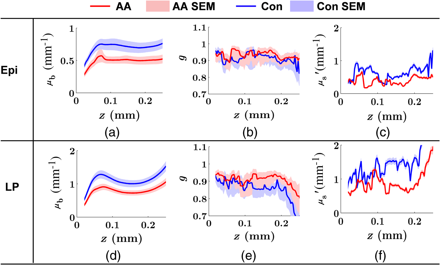

Next, we examined the ultrastructural changes quantified based on the W–M model. Both epithelium and LP from AA patients showed a higher $D$ compared with that of control patients [Figs. 6(a) and 6(d)]. Epithelium showed a better contrast within the top 100-μm depth, whereas in LP, the greatest change was noted in deeper tissue $>200\mu \text{m}$ [Figs. 6(a) and 6(d)]. $L_n$ did not appear to be appreciably different in epithelium between control and AA, but in LP, AA patients had elevated $L_n$ for tissue depths around 100 to 200 μm. To compare the RI fluctuation magnitude, Figs. 6(c) and 6(f) show $B_n$ ($r_d=35\mathrm{nm}$) as a function of tissue depth. The value of 35 nm is the lower limit of length scale sensitivity of ISOCT, beyond which ISOCT can no longer detect ultrastructural alterations.²³ We note that at $r_d=35\mathrm{nm}$, the RI fluctuations are weaker in AA group than in control [Figs. 6(c) and 6(f)].

Fig. 6

Depth-resolved ultrastructural properties quantified in CRC field carcinogenesis. The parameters were compared between control (Con) and AA groups separately in (a–c) epithelium (Epi) and (d–f) LP. The shadow areas show the standard error of the mean (SEM). $B_n$ is calculated at $r_d=35\mathrm{nm}$ by using the mean value of $A_n$, $D$, and $L_n$ according to Eq. (1).

5.4.

Depth-Resolved Changes in CRC Field Carcinogenesis

The most significant optical and ultrastructural alterations in the epithelium and LP may occur at different depths. To identify the locations of the alterations in the epithelium and LP, we plotted the relative change in the optical and ultrastructural properties between AA to control groups and the corresponding $p$-values as a function of depth (Fig. 7). Because ${\mu }_{\mathrm{b}}$ and $D$ are two directly measured depth-resolved quantities, we used them as our representative markers. In epithelium, the contrast for $D$ reached a maximum around $\sim 65\mu \text{m}$ in depth [Fig. 7(a)], and the depth range, where the difference was significant ($p<0.05$), was from 50 to 75 μm [Fig. 7(c)]. In LP, the optimal contrast for $D$ was from $\sim 200$ to 250 μm [Figs. 7(b) and 7(d)]. The $p$-values for ${\mu }_{\mathrm{b}}$ are below 0.05 for all depths in both compartments.

Fig. 7

Percent change and $p$-values of $D$ and ${\mu }_{\mathrm{b}}$ from AA group to control (Con) group, in (a and c) epithelium (Epi) and (b and d) LP. The dashed lines are labeled 5% level. The red bars on $x$-axis show the depth range where the averaged values are calculated for comparison in Figs. 8 and 9.

Having identified the location of the most significant alterations, we next examined whether the alterations parallel the progression of the severity of field carcinogenesis and the risk of carcinogenesis. As discussed in Sec. 4, we considered four groups of patients depending on colonoscopic findings: patients with no neoplastic lesions, patients with HPs (most carrying no malignant potential), patients with non-AAs, and finally those with AAs. Figure 8 shows the averaged values of the optical properties from 40 to 90-μm depth in epithelium and 200 to 250 μm in LP. Overall, the change in most of the optical properties paralleled the CRC risk from control patients to those with AAs and was consistent in both epithelium and LP: ${\mu }_{\mathrm{b}}$ progressively decreased, $g$ increased, ${\mu }_{\mathrm{s}}$ and ${\mu }_{\mathrm{s}}^{\prime }$ decreased. While the change in the majority of the parameters reached statistical significance, a few parameters failed to reach $p<0.05$ significance level (Fig. 8). This could be due to the biological variability with our finite sample size.

Fig. 8

Bar plots of optical properties in CRC field carcinogenesis. The averaged ${\mu }_{\mathrm{b}}$ (a and e), $g$ (b and f), ${\mu }_{\mathrm{s}}^{\prime }$ (c and g), and ${\mu }_{\mathrm{s}}$ (d and h) were compared in four groups: control (Con), hyperplastic polyps (HPs); adenoma (Ade); and AA. Data were averaged at depth 40 to 90 μm in epithelium (Epi) and 200 to 250 μm in LP. *$p<0.05$.

Figure 9 plots the average values of the ultrastructural properties $D$, $L_n$, and $B_n$ ($r_d=35\mathrm{nm}$) assessed from the same locations as in Fig. 8. Both in epithelium and LP, $D$ increased and $B_n$ ($r_d=35\mathrm{nm}$) decreased progressively paralleling the risk of CRC from control patients to those with AA. There were no obvious trends for $L_n$. The values of $L_n$ were around 1 μm.

Fig. 9

Ultrastructural properties in CRC field carcinogenesis. The averaged $D$ (a and d), $L_n$ (b and e), and $B_n$ ($r_d=35\mathrm{nm}$) (c and f) were compared in four groups: control (Con), HPs; adenoma (Ade); and AA. Data were averaged at depth 40 to 90 μm in epithelium (Epi) and 200 to 250 μm in LP as marked in Fig. 7. *$p<0.05$.

5.5.

Optical and Ultrastructural Properties in PC Field Carcinogenesis

A similar approach and data analysis were used to analyze the optical and ultrastructural alterations occurring in PC field carcinogenesis. While the pancreatic duct shows the diffuse carcinogenesis, directly instrumenting the pancreatic duct is fraught with complications. Several groups have shown that the peri-ampullary duodenum shares profound molecular changes (mutations/methylation) with the pancreatic duct in patients harboring PC.^83,84 Thus, we chose the peri-ampullary duodenum as the surrogate site for PC field carcinogenesis. The patients were categorized into two groups as shown in Table 3: control (no pancreatic neoplasia) and pancreatic adenocarcinoma (AC) according to the pathology report after the endoscopic examination.

Table 3

PC study: patient characteristics.

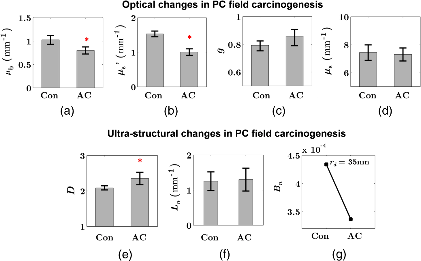
Because the structure of duodenal villi is considerably more complicated than the cryptal morphology of rectal mucosa, the separation of epithelium and LP in the duodenal biopsies was impractical. Thus, we calculated the optical and ultrastructural properties of the duodenal biopsies as a combined effect of both components. Depth-resolved optical and ultrastructural changes from PC to control patients were plotted in Fig. 10. Using the similar method in CRC field carcinogenesis, we also identified significant alterations at two depth segments at about 30 to 80 μm and 170 to 220 μm in PC patients based on the changes in ${\mu }_{\mathrm{b}}$ and $D$ (Fig. 11). The averaged values of the optical and ultrastructural properties from the first segment are plotted in Fig. 12. A decrease in ${\mu }_{\mathrm{b}}$, ${\mu }_{\mathrm{s}}^{\prime }$, and $B_n$ ($r_d=35\mathrm{nm}$) and increase in $D$ and $g$ were observed in PC field carcinogenesis, which is consistent with the similar changes in CRC field carcinogenesis.

Fig. 10

Depth-resolved optical and physical properties of duodenum samples in pancreatic cancer (PC) field carcinogenesis. Comparison of control (Con) group and adenocarcinoma (AC) group for ${\mu }_{\mathrm{b}}$, ${\mu }_{\mathrm{s}}^{\prime }$, and $g$ (a–c) and $D$, $L_n$, and $B_n$ ($r_d=35\mathrm{nm}$) (d–f). The shadow areas show the standard errors of the mean (SEM).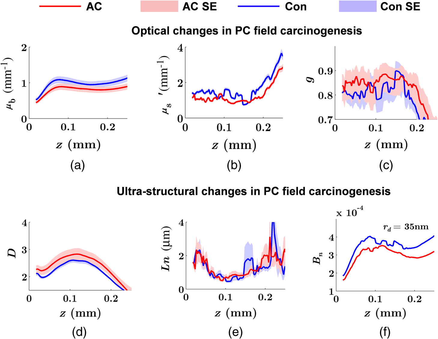

Fig. 11

(a) Relative changes and (b) $p$-values of $D$ and ${\mu }_{\mathrm{b}}$ from adenocarcinoma (AC) group to control (Con) group in duodenal specimen. The dashed lines are labeled 5% line. The red bars on $x$-axis show the depth range where the averaged values are calculated for comparison in Fig. 12.

Fig. 12

Bar plots of (a–d) optical and (e–g) ultrastructural properties in PC field carcinogenesis. Con: control; AC: adenocarcinoma. Data were averaged at depth 30 to 80 μm. *$p<0.05$.

5.6.

Mechanisms for Intracellular and Extracellular Ultrastructural Changes

In the previous sections, we investigated the histological location (epithelium versus LP and depth) and physical nature [$B_n(r_d)$] of the optical/ultrastructural changes in CRC and PC fields carcinogenesis. The next question is what causes these physical changes in terms of specific intra- and extracellular structures? As mentioned above, chromatin clumping and collagen cross-linking are two of the most common structural hallmarks in cancer. Both events are expected to lead to a shift of structural length scales to larger sizes in accordance with the change in $B_n(r_d)$ observed by ISOCT. Therefore, we tested whether those events could also play a role in the ultrastructural alterations in field carcinogenesis.

To alter the chromatin structure, we chose an aggressive variant of colon cancer cell line, CSK knockdown HT-29 cells, applied VPA to inhibit HDACs, and introduced chromatin relaxation. Chromatin compaction is partly mediated by HDACs,⁸⁵ a class of enzyme that allows the DNA to wrap around the histones. VPA is a drug known to have the effect of inhibiting HDACs, so that the VPA-retreated chromatin is less compacted.⁸¹ The treatment was performed according to the established protocol with VPA concentration of 1.5 mM, as described in Sec. 4.5. The ISOCT measurements were performed on cell pellets (cell deposition after centrifuge) after 4-h treatment ($n=9$ for both 0 and 1.5 mM VPA treatments), at which time point the effect of VPA approximately reached its maximum.⁸⁶ Figure 13(a) shows a decrease in $D$ for cells treated with VPA. This suggests that the chromatin compaction manifests itself as an increase in $D$, in agreement with the field carcinogenesis alteration observed by ISOCT in the rectal epithelium.

Fig. 13

$D$ changes induced by (a) the de-compaction of chromatin structure and (b) the cross-linking of the collagen fiber network. Valproic acid (VPA) was used to inhibit histone deacetylases (HDACs) to relax chromatin. Lysyl oxidase (LOX4) was used to induce cross-linking of the collagen fibers. $D$ analysis was performed on the signal averaged within the top 80 μm of the samples. *$p<0.05$, **$p<0.001$.

To introduce changes in ECM, we used collagen fiber models of ECM and applied LOX to induce the collagen cross-linking. LOX alters collagen structure by promoting collagen cross-linking.⁸² The gels were incubated with LOXL4 with increasing final concentration from 150 to $350\mu \text{g}/\mathrm{mL}$. As in Fig. 13(b), $D$ increased progressively from $2.1\pm 0.06$ in control gels to $2.7\pm 0.18$ in gels treated with $350\mu \text{g}/\mathrm{mL}$ LOXL4 ($n=12$ for each treatment concentration). This experiment demonstrated that ECM collagen cross-linking induces an increase in $D$ in agreement with the field carcinogenesis alteration observed by ISOCT in rectal stroma.