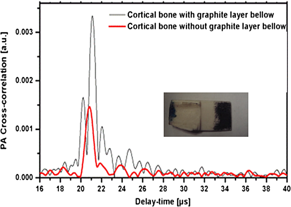
2.1.

Coded Excitation PA and US Imaging

The use of coded excitation signals in US imaging and its benefits are discussed elsewhere.⁴⁵ The appropriate method for our application is the use of a linear frequency modulation signal, which generates high-SNR enhancement and linear frequency spectrum in the selected range. The instantaneous frequency is defined as

Other factors such as acoustic attenuation and transducer transfer function affect the sinc-function shape of the US signal. In addition to these factors, the energy conversion process in PA tends to dominate the signal shape.⁴⁶ By employing reference signals from a perfect reflector in US and a homogeneous known absorber in PA, the effects of transducer and instrumentation can be compensated for. Here, spectral analysis is the main goal and therefore a suitable frequency range should be selected to optimize the response depending on the average size of the scatterers. A middle stage in the spectral analysis is the time-gating of the time-domain cross-correlation signal and transforming back into FD. Time-gating provides the facility to separate the various parts of the signal generated by direct reflection from cortical and other overlayers and through backscattering from the trabecular layer.

2.2.

Combined PA and US Coregistration Experimental Set-up

The experimental set-up is depicted in Fig. 1(a). This set-up facilitates separate PA and US tests at the same coordinate location of bone samples. Optical excitation of the PA probe was generated using a CW 800-nm diode-laser (Jenoptik AG, Jena, Germany). The laser driver was controlled by a software function generator to modulate the laser intensity. A collimator was used to generate a collimated laser beam with 2-mm spotsize on the sample. The choice of 800 nm was made for maximum penetration depth in bone tissue in the near-IR region.⁴⁷ A 3.5-MHz focused ultrasonic transducer was used for transmitting the US signal (V382, Olympus NDT Inc., Panametrics, Waltham, Massachusetts). This transducer has 0.5 in. element size and 1 in. focal length. Beam width at half maximum was estimated to be 0.87 mm.⁴⁸ The sensitivity of this transducer was measured with a calibrated hydrophone and was found to be $31.8\mu \mathrm{V}/\mathrm{Pa}$.⁴⁹ By employing the reciprocity property of piezoceramics, we could estimate the transmitted US intensity generated by this transducer. The RMS US amplitude was 2.25 mV. This signal was 40 dB amplified by the RF power amplifier (411LA ENI Co., Rochester, New York, 10 W) connected with the transducer which thus generated a pressure of 72 kPa at the focal zone or $\mathrm{34,800}\mathrm{kW}/{\mathrm{cm}}^2$ in water.

Fig. 1

(a) Block diagram of combined (“coregistration”) photoacoustic (PA) and ultrasound (US) experimental set-up. (b) Matched filter algorithm used to generate A-scans; $r(t)$: reference signal (Chirp), $s(t)$: signal detected by the ultrasonic transducer, FFT and IFFT: fast Fourier transform and inverse FFT, Z*: complex conjugate.

Backscattered pressure waves were detected with a 2.2-MHz focused transducer (V305, Olympus NDT Inc., Panametrics, Waltham, Massachusetts) of 0.75 in. diameter and 1 in. focal length. The beamwidth was estimated to be 0.9 mm.⁴⁸ Different transducers are employed to provide the possibility of testing a wider range of frequencies by switching the transducers, however, in this report, the 2.2-MHz transducer was used as receiver and the 3.5-MHz transducer was used as transmitter. Both transducers provide good sensitivity in the selected frequency range of the chirps and the effect of transducer and instrumentation has been compensated by normalizing with reference US and PA spectra as explained further on.

The bone sample and the transducer were located in a water container for acoustic coupling. The system was designed for back propagating detection and there was a $\sim 27\mathrm{deg}$ angle between the laser beam and each transducer’s center line. The point of incidence of the laser beam was perpendicular to the water surface. The laser beam was further used to adjust the focal point of both transducers on the same spot on the sample. The US focal beam widths of both transducers were very close and $<1\mathrm{mm}$. In the experiments, we used stepsizes $\ge 1\mathrm{mm}$ between the measured A-scans to prevent overlapping between measurements. According to the literature $<50\%$ cross-sectional overlap between regions of interest is required to ensure independent data.²⁹

Data acquisition and signal processing were performed in the PC using LabView software. Linear frequency modulation chirps and a matched filtering method were employed to generate A-scans.⁴⁶ Figure 1(b) describes the signal generation pathway of matched filtering using the fast Fourier transform module (FFT). The cross-correlation (CC) signal was calculated by multiplying the Fourier transform of the detected signal with the complex conjugate of the Fourier transform of the reference signal. In addition to the in-phase CC, the quadrature CC was also calculated by eliminating the negative frequencies and making the signal analytic. In the end, the inverse FFT operator provided the CC in the time domain. Although the existence of real and imaginary parts generates a separate phase channel,⁵⁰ the phase signal was not used in this study because backscattering quantification was performed using integrated power spectrum. The chirp duration was 1 ms and A-scans were generated by averaging over 80 to 180 signal chirp records. The chirp bandwidth was adjusted to maximize the PA and US SNRs sequentially. In the PA (US) the frequency range used was 300 kHz to 2.6 MHz (300 kHz to 5 MHz).⁴⁶

The employed laser power was 1.6 W and the beam spotsize after the collimator was 2 mm, which generates a fluence of $50\mathrm{W}/{\mathrm{cm}}^2$. Despite the large fluence, its magnitude is under the maximum permissible exposure (MPE) due to the very short radiation time.^49,51 The chirps were transmitted in 10-ms batches, which correspond to MPE of $55\mathrm{W}/{\mathrm{cm}}^2$. ($\mathrm{MPE}=1.1{\mathrm{C}}_A{t}^{1/4}\mathrm{J}/{\mathrm{cm}}^2$, ${\mathrm{C}}_A=1.58=>\mathrm{I}=\mathrm{MPE}/t=55\mathrm{W}/{\mathrm{cm}}^2$).

The samples used in this work were goat rib bones (Canadian goat, Caprine). The samples were defatted by immersing in water for 3 weeks leading to natural soft tissue decomposition. Then, they were cleaned and washed and left to get completely dried. Also, a human trabecular bone (SteriGraft, San Antonio, Texas) from calcaneus was used for testing the cancellous bone alone. To perform decalcification simulating osteoporosis, 0.5-M ethylenediaminetetraacetic acid (EDTA) solution was used. This solution produces very slow and gentle demineralization and is extensively employed to simulate osteoporosis in bone tissue due to dissolving the bone minerals while leaving the organic components intact.^52,53 The extent of demineralization depends on solution concentration and exposure duration as well as exposed area and bone compactness. More details are given in Sec. 3.

3.1.

PA Response of a Cortical Layer

One experiment was introduced to demonstrate the possibility of detecting PA signals from below dense cortical layers. PA signals from a thin layer of goat cortical bone ($1.5\pm 0.06\mathrm{mm}$) between two adjacent locations were compared, such that in one case the underlayer was stained with graphite (Fig. 2). The strong peak due to the graphite layer indicated the penetration of laser light and the possibility of detecting PA signals below the cortical layer. Comparing the amplitude of the detected signal from cortical bone with the signal from the known sample, the bone absorption coefficient could be estimated. Bone absorption depends on bone compactness as well as concentration of the chromophores in the bone. Here, the frequency bandwidth is not in a range sensitive to the cortical bone porosity and therefore the response would be comparable to the signal from a flat surface with homogenous absorption. To extract the absorption coefficient, the photoacoustic induced pressure is normally approximated as^54,55

Fig. 2

PA signal from a thin goat cortical bone ($1.5\pm 0.06\mathrm{mm}$) with and without graphite sublayer.

Here, $c_a$ and $c_s$ are the SOS in the bone and coupling medium (water), respectively, and ${\rho }_a$ and ${\rho }_s$ are the density of the bone and coupling medium, respectively. In this analysis, the thermal diffusion and shear waves in the bone are considered to be negligible and the SOS is in the perpendicular direction to the transducer. The value of the Grüneisen coefficient of cortical bones is considered to be 0.68 [with thermal expansion coefficient $88\times {10}^{-6}{\mathrm{K}}^{-1}$ (Ref. 56), specific heat $1.33\mathrm{J}·{\mathrm{g}}^{-1}·{\mathrm{K}}^{-1}$ (Ref. 57), and SOS $3198\mathrm{m}/\mathrm{s}$; also the bone density is considered to be $1990\mathrm{kg}/{\mathrm{m}}^3$ (Ref. 58)]. We used a diluted solution of “Lamp Black” water color (Cotman Water Colours, Winsor & Newton, London, United Kingdom) as reference absorber. The absorption coefficient of the solution was measured optically by comparing the power of a CW laser passing through an empty 2-mm-glass spectrophotometer cell (cuevette) (Starna Cells Inc, Atascadero, California) and laser power passing through a cuevette filled with the solution. Using Beer’s law the absorption coefficient of the diluted water color was measured to be $3.18{\mathrm{cm}}^{-1}$. The Grüneisen coefficient of diluted aqueous solution was estimated by the empirical formula; $\mathrm{\Gamma }=0.0043+0.0053T$, where $T$ is the room temperature in deg Celsius. The PA measurement of water color solution was performed using a container with a very thin plastic surface on one side.^49,59 The cross-correlation amplitude is proportional to the detected pressure, thus, by comparing the peak amplitude of bones with the peak amplitude from the reference absorber and implementing the correction factor described in Eq. (6) we can estimate the absorption coefficient of bone. In this experiment, the laser power and all other parameters remain identical. This experiment yielded bone absorption coefficients between 0.08 and $0.22{\mathrm{cm}}^{-1}$ at 800-nm wavelength. These values are consistent with published literature values.^47,60,61

3.2.

PA and US Signals from a Human Trabecular Bone

In another experiment, PA and US backscattering signals from a trabecular bone block of human calcaneus were analyzed. The human bone lost its marrow and had reduced lipid elements following the cleaning procedure; however, the minerals were left intact. The size of the bone was $15.7\times 15.7\times 35{\mathrm{mm}}^3$. Its apparent density was estimated to be $360\mathrm{mg}/{\mathrm{cm}}^3$, a value derived by weighing the bone and dividing the weight by its volume. On one side of the bone some holes were drilled, whereas the other side remained intact [Fig. 3(a)]. The distance from the holes to the tested surface was $\sim 3\mathrm{mm}$. To eliminate the effect of the transducer and other instruments, the spectra of PA and US signals were normalized with reference signals conforming theoretically to Eqs. (1) and (2). An ideal reflecting material for US backscattering reference was a polished metal (here aluminum) surface, and for PA, a thick-homogeneous absorber (plastisol) with a known absorption coefficient of $9{\mathrm{cm}}^{-1}$. The backscattered PA and US spectra from the abovementioned ideal reflector/absorber are shown in Fig. 3(b), where the ordinates are not to scale. A similar normalization procedure was performed for all our experiments.

Fig. 3

(a) Human trabecular bone sample. (b) Reference PA and US spectra used for respective normalizations. (c) Spatially averaged PA spectra (6 points) of trabecular intact bone and over the drilled region. (The average standard deviations divided by spectral amplitudes were 22% and 23%, respectively). (d) Spatially averaged US spectra (6 points) of trabecular intact bone and over the drilled region. (The average standard deviations divided by spectral amplitudes were 19% and 22%, respectively.) (e) PA cross-correlation envelope of trabecular bone over the drilled hole and after it was filled with black cylindrical rubber beneath 3 mm of cancellous bone. (f) US counterpart of (e) at the same point. (g) and (h) show the PA and US cross-correlations depicted in (e) and (f) in logarithmic scale respectively to highlight minor changes.

The PA and US spectra were averaged over measurements at six points on the intact bone and six points over the holes. To make a comparison between the changes in the PA and US spectra, the centroids and spectral powers of US and PA signals in the same frequency range, 0.3 to 2.6 MHz, were considered. The spectral power is defined by the integrated power spectrum in Eq. (2), and the spectral centroid is defined as

Figures 3(c) and 3(d) compare the averaged PA and US spectra for the two cases. There is no meaningful change between the spectra in the two cases compared with the signal variation from point to point. The integrated spectrum has been reduced by 5.1% and 3.7% over the hole for PA and US cases, respectively. The centroids of the PA spectra are $1890\pm 28$ $(1918\pm 23)\mathrm{kHz}$ for intact bone (over the hole), and $1459\pm 72$ $(1724\pm 63)\mathrm{kHz}$ for their US counterparts over the common frequency range 0.3 to 2.6 MHz. It can be seen that: (1) the centroid of the averaged spectrum has been increased by removing part of the trabecular bone below 3 mm for US and also PA (the change in PA centroid is statistically significant with 85% confidence based on $t$-test); (2) The change in the centroid is much smaller for the PA spectrum than for its US counterpart; and (3) the US centroid frequencies are lower than PA centroids. It should be mentioned that the PA low-pass effect has been accounted for after normalization with the homogeneous absorber, otherwise we would expect to have higher centroids for US spectra than for PA. The reason for the three above-mentioned observations can be attributed to ultrasonic attenuation in bone media, which increases with frequency and causes higher frequencies to be damped in the case of the intact bone compared with the drilled bone. US signals undergo greater high-frequency reduction than PA signals due to the double transmission path of the US backscattered signal.

Subsequently, in another experiment, the PA and US signals over the hole were compared with the signals after the hole was filled with a black rubber absorber (cylinder). This experiment demonstrates that a laser-induced US signal can still be generated even below 3 mm of trabecular bone. Otherwise, the signals from this depth would be mostly attributed to the multiple scattering of US in the random scattering medium. The PA signals with and without the black rubber cylinder are compared in Fig. 3(e). It can be seen that by inserting the cylinder, a new peak appears in the corresponding depth with minimal changes to the first peak of the signal prior to the insertion. Figure 3(f) shows the US counterparts of the signals in Fig. 3(e). As shown, inserting the black rubber cylinder below 3 mm of trabecular layer has almost no effect on the US signal. This should be attributed to the large-acoustic attenuation of bone in the employed frequency range, note that due to echo measurements the attenuation depth is 6 mm in this case. The PA and US normalized power spectra in the same frequency range over the intact bone are compared in Figs 4(a)–4(c) for three different points. The PA and US spectra were normalized by use of the experimental signals from the perfect reflector/absorber as described above. The coherent backscattering effect can be detected in the presence of resonance peaks in both PA and US spectra. Coherent backscattering is considered as “unmistakable signature of multiple scattering”³⁸ and can be applied to estimate the scattering mean-free time in the bone, which corresponds to the distance between scatterers (trabeculae).³⁸ Therefore, we can expect to have similarities in the interfering frequencies of the two modalities. From the figures, we can see that PA generates more peaks because PA interferences are not only generated by coherent PA signals from trabeculae but also from their echoes: light reaches simultaneously all absorbing/PA signal generating targets which also respond simultaneously, thereby preserving their individual response character on a short (one-way) transit time scale to the transducer. The US excitation penetrates deeper than optical irradiation because the latter undergoes depth-dependent absorption attenuation, and it generates responses upon arrival at each target sequentially, which takes longer round-trip times. The US generated echoes from all layers with round-trip time delays add structure to the low-frequency end of the spectrum. The result is the PA- and US-generated spectra are heavily weighed at high and low frequencies, respectively, as seen in Fig. 3(b) and are, therefore, complementary. It is important to add that the attenuation of US signal from deeper layers is mainly a function of structural properties of the medium, whereas attenuation of the PA signal is a function of molecular composition in addition to the medium structure. In summary, in the combined US and PA signals both composition and structure are important factors in shaping the frequency spectra. Several similar structures appear in the mid-range of both spectra. For instance, the resemblance of peak and trough structure in the frequency range 1.5 to 2 MHz in Fig. 4(a) indicates that in both cases coherent backscattering is strongly correlated with the scattering mean-free time in the bone, which corresponds to trabecular thickness and separation. However, due to the frequency dependence of the PA signal phase, the phases at the peaks and troughs do not have a direct correspondence. The normalized PA spectrum specifically shows an increase with frequency, which is due to the distribution of trabeculae interdistances.

Fig. 4

Comparison of PA and US spectra normalized with reference spectra for three different locations (a), (b), and (c) on the intact part of the cancellous bone in Fig. 3(a).

3.3.

PA and US Signal Validation Using Microcomputed Tomography

In another experiment, the PA and US signals from a set of four defatted goat rib bones were analyzed with the goal to test PA and US sensitivity to demineralization. As shown in Fig. 5(a) seven points with 1-mm distance between them were tested at different demineralization stages. The demineralization solution was made by diluting 50 ml of EDTA solution (0.5 M, $\mathrm{pH}=8$) in equal volume of distilled water, which generates a pH of 7.7. The EDTA solution produces very slow and gentle decalcification and its mild solution ($\mathrm{pH}\le 8$) has been widely used in the literature for simulating artificial osteoporosis.^52,53,62 The four bone samples were kept in the solution for 10, 20, 30, and 40 h of demineralization, respectively. The samples were attached to Lego blocks to ensure the tests had been performed at the same locations on the ribs before and after demineralization. The fourth sample was demineralized without removal of the bone, to ensure successive measurements from exactly the same points. To validate the US and PA results with an established method of BMD assessment, the samples were also imaged with microcomputed tomography (μCT). The μCT scans were performed in the air using a SkyScan system (SkyScan, Belgium) with the settings: 60 kV, 167 μA, 0.25 step size, four frame average, $4000\times 2672\text{pixel}$ matrix, and a $5\text{-}\mu {\mathrm{m}}^2$ pixel size. Total scan time was 2.5 h. Images were reconstructed using a modified Feldkamp cone-beam algorithm.⁶³ Subsets of the data were created which included all bone parts within the rib and spanned the region between the two arrows in Fig. 5(a). That section consists of 760 μCT slices. Three analysis regions were determined on the rib sample: middle region of the dorsal cortical shell, trabecular bone of the rib, and both of these tissues together. The μCT slices of the fourth sample in three directions are shown before demineralization, Fig. 5(b), and after 40 h of demineralization, Fig. 5(c). The ensemble-averaged PA and US cross-correlation signals of the fourth sample are shown in Figs. 5(d) and 5(e), respectively. These signals show the variation of averaged US and PA signals from cortical and trabecular layers of intact and 40-h demineralized bone. It can be observed that the variation of the reflected US signal from the cortical layer is minor, while the first peak of PA signal changed significantly. On the other hand, in the deeper layers the PA signal increased with demineralization. This can be explained by considering that demineralization reduces optical scattering and thus may allow optical energy to access deeper layers more effectively.

Fig. 5

(a) A goat rib sample with measurement region, points 1 to 7, shown between arrows. Three μCT slice images of the goat bone in three orientations: (b) before and (c) after 40-h demineralization with EDTA solution. The ensemble averaged over the 7 points (d) PA and (e) US envelope cross-correlation signals before and after 40-h demineralization.

Time gating has allowed separation of the reflected US and back-propagated PA signals from the cortical layer. The spectra of these signals were normalized with the respective reference spectra similar to the previous experiment. Integrating over the frequency range, the US IRC and PA AIB from the cortical layer were calculated [Eq. (2)]. Likewise, by time gating the cortical- and trabecular-backscattered signals together, the total integrated US and PA backscattering coefficients can be calculated. Variations of the integrated backscattered signals versus BMD of the cortical and the combined cortical and trabecular volume of interest derived from μCT are shown in Figs. 6(a) and 6(b). For the third sample, the extent of trabecular demineralization was too high after 30 h and therefore this sample was excluded from the total cortical and trabecular result statistics after demineralization. The trabecular region of the fourth sample was less demineralized compared with the third sample despite the fact that they were demineralized for 40 and 30 h, respectively. The main difference between the demineralization process of the forth sample and that of the others was that this rib bone was located horizontally in the demineralization tank while other samples were hung in the solution. The linear regressions of the measurements show the degree of correlation and sensitivity of PA and US to changes in bone density in the cortical and cancellous regions. Comparison of the slope of the lines demonstrates the higher sensitivity of PA to BMD variations in the cortical part. As seen in the figures, the variances are quite large which is due to the nature of the experiment and variability and inhomogeneity of real bone tissue, rather than the result of low SNRs. Figures 7(a) and 7(b) compare the point-by-point variation of US and PA backscatter from cortical layers of the first and second sample before and after 10 and 20 h of demineralization, respectively. The comparison between the point-by-point changes and variations due to demineralization demonstrate the main challenge of assessment of biological tissue. The sensitivity of each modality should be able to dominate the natural variation of properties in the tissue and yield meaningful statistical analysis. Strictly speaking, this is achieved only with the PA signal after 20 h of demineralization. Using a statistical $t$-test for the results, the majority of the integrated PA-backscattered measurements demonstrates statistically significant reduction with 90% confidence. Table 1 shows the changes of BMD and integrated PA back-propagation and US reflection from the cortical layer. Except the first sample after 10 h of demineralization, in all other PA cases, the changes were significant while none of the US results show adequate sensitivity to BMD variation in the cortical layer.

Fig. 6

The integrated (a) PA and (b) US-backscattered signals of cortical and combined cortical and trabecular bone versus BMD of volume of interest as obtained from μCT analysis.

Fig. 7

Point by point US and PA-backscattered signal variations from samples (a) 1 and (b) 2, before and after 10- and 20-h demineralization, respectively.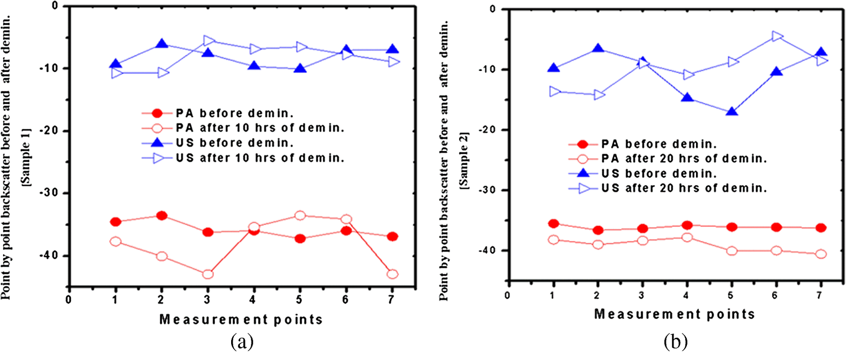

Table 1

Changes of integrated photoacoustic (PA) and ultrasound (US) backscatter parameters due to bone demineralization (artificial osteoporosis).

The variation of US IRC and PA AIB (cortical layer only) of eight samples versus hours of demineralization is shown in Fig. 8. The four cortical samples were the same ones described before (rib cortical) and another four measurements were performed from the other side of the same samples. The signal variation was larger across the opposite sides of the ribs compared with different locations on the same side. Figure 8 demonstrate that the average change of PA AIB in the cortical layer is significantly larger than the standard deviation of the properties at each stage, while this is not the case with US IRC (cortical layer). Hence, Fig. 8 is consistent with the statistical analysis described in Table 1, over a larger set of samples.

Fig. 8

The variation of PA and US-backscattered signal from the cortical layer (in US it is the reflection parameter IRC) versus hours of demineralization.