Incoherence-based optimal selection of independent measurements in diffuse optical tomography

Calvin B. Shaw; Phaneendra K. Yalavarthy

doi:10.1117/1.JBO.19.3.036017

21 March 2014 Incoherence-based optimal selection of independent measurements in diffuse optical tomography

Calvin B. Shaw, Phaneendra K. Yalavarthy

Author Affiliations +

Journal of Biomedical Optics, Vol. 19, Issue 3, 036017 (March 2014). https://doi.org/10.1117/1.JBO.19.3.036017

Abstract

An optimal measurement selection strategy based on incoherence among rows (corresponding to measurements) of the sensitivity (or weight) matrix for the near infrared diffuse optical tomography is proposed. As incoherence among the measurements can be seen as providing maximum independent information into the estimation of optical properties, this provides high level of optimization required for knowing the independency of a particular measurement on its counterparts. The proposed method was compared with the recently established data-resolution matrix-based approach for optimal choice of independent measurements and shown, using simulated and experimental gelatin phantom data sets, to be superior as it does not require an optimal regularization parameter for providing the same information.

1. Introduction

Near-infrared (NIR) diffuse optical tomography is an emerging imaging modality with applications including breast cancer imaging¹^,² and brain function assay.¹^,³ The interrogating medium in diffuse optical tomography is NIR light in the spectral range of 600 to 1000 nm. A finite set of boundary measurements are acquired in NIR tomography that in turn is used to reconstruct the internal distribution of optical properties.⁴^,⁵ The NIR light is delivered through optical fibers and the transmitted light is collected typically through the same fibers, which are in contact with the surface of the tissue. The distribution of optical properties of the tissue are reconstructed using measured boundary data with the help of model-based iterative algorithms.⁴

The inverse problem encountered in diffuse optical imaging is usually an underdetermined problem with a high correlation between measurements because of the diffusive nature of light propagation. Optimization of data-collection strategy has been an active area of research,⁶^–¹¹ where the recent emphasis is on independent measurement selection strategy.¹⁰^,¹¹ The data-collection optimization plays an important role in any imaging system design, where acquiring the independent measurements can reduce significantly the data-collection time, in turn reducing the total imaging protocol time. More over, this kind of optimization can lead to faster frame rates especially in dynamic imaging scenarios,¹²^,¹³ where the emphasis is to achieve the video-rate. Most diffuse optical imaging systems utilize the photomultiplier tubes (PMTs) for detection of light due to their high gain and sensitivity,⁵^,¹⁴ making simultaneous detection channels dependent on number of PMTs used, where the cost of the imaging systems largely depends on the detection channels. The reduction in the number of measurements without compromising the image quality will also lead to cost effective systems and such testing of detection arrays could be achieved by these studies without physically building them.

The measure of incoherence has been extensively studied in the field of compressive sensing,¹⁵ which is defined as the maximum absolute value of the cross-correlations between the columns of a matrix. In this work, we present a framework that uses the measure of coherence on the set of rows of the sensitivity (Jacobian) matrix to decide the coherent (dependent) and incoherent (independent) measurements encountered in diffuse optical imaging. In order to show the effectiveness of the proposed method initially the data resolution-based measurement selection method,¹¹ which was established recently as the state of the art method for predicting if a specific measurement is independent or not, is taken up to show the dependence of data resolution matrix on the regularization parameter. The proposed method was compared with the random selection of measurements using simulated and experimental gelatin phantom data to show that it provides an optimal selection of independent measurements. The discussion is limited to two-dimensional (2-D) frequency-domain data case, where the collected boundary data is the natural logarithm of amplitude and the phase information and the unknown parameters to be reconstructed are the optical absorption and reduced scattering coefficients.

2. NIR Diffuse Optical Tomography: Forward Problem

In the frequency domain, the NIR light propagation in thick biological tissues like breast and brain can be modeled using diffusion equation,⁴ given as

Eq. (1)

- \nabla . [D (r) \nabla Φ (r, ω)] + [μ_{a} (r) + \frac{i ω}{c}] Φ (r, ω) = Q_{o} (r, ω),

where

μ_{a} (r)

represents the optical absorption coefficient and

D (r)

, the optical diffusion coefficient, which is defined as

D (r) = \frac{1}{3 [μ_{a} (r) + μ_{s}^{'} (r)]}

, where

μ_{s}^{'} (r)

is the reduced optical scattering coefficient, which is defined as

μ_{s}^{'} = μ_{s} (1 - g)

with

μ_{s}

and

g

representing the scattering coefficient and anisotropy factor respectively. The isotropic light source is represented by

Q_{o} (r, ω)

and the speed of light in the tissue as

c

. The photon fluence density at a given position

r

is represented by

Φ (r)

and the light modulation frequency is given by

ω

(

ω = 2 π f

with

f = 100 MHz

). The finite element method (FEM) is used to solve Eq. (1) to generate the amplitude and phase measurements for a given distribution of the absorption

μ_{a} (r)

and diffusion [

D (r)

] coefficients.¹⁶ A type-III boundary condition is incorporated to account for the refractive-index mismatch at the boundary.⁴ This forward model is used repeatedly in an iterative framework to estimate the optical properties of the tissue under investigation.⁴^,¹⁶^,¹⁷

3. NIR Diffuse Optical Tomography: Inverse Problem

The inverse problem primarily deals with the estimation of optical absorption ( $μ_{a}$ ) and diffusion ( $D$ ) coefficients from the amplitude [ $\ln (I)$ ] and phase ( $θ$ ) boundary measurements using a model-based approach. This is accomplished by matching the experimental measurements ( $y$ ), which is the natural logarithm of the amplitude and phase of the experimental data with the model-based ones [ $F (D, μ_{a})$ ] iteratively in the least-squares sense over the range of $D$ and $μ_{a}$ . Even though $D$ and $μ_{a}$ are the parameters that are being estimated, the $μ_{a}$ and $μ_{s}^{'}$ images are shown as the final output, which are spectroscopically meaningful to interpret. This minimization problem is solved using the Levenberg–Marquardt (LM) optimization scheme¹⁸ and the objective function to be minimized is defined as

Eq. (2)

Ω = \min_{D, μ_{a}} {‖ y - F (D, μ_{a}) ‖}^{2} .

The first order condition (setting the first derivatives with respect to $D$ and $μ_{a}$ to zero)¹⁸ to minimize Eq. (2) results in an iterative update equation of the form,

Eq. (3)

(Δ D^{i}, Δ μ_{a}^{i}) = J^{T} {{[JJ}^{T} + λ I]}^{- 1} δ^{(i - 1)} .

Here, $Δ D^{i}$ and $Δ μ_{a}^{i}$ represent the update of the optical diffusion and absorption coefficients at the $i$ ’th iteration, respectively, $δ = y - F (D, μ_{a})$ is defined as the data-model misfit, $J$ as the Jacobian or the sensitivity matrix, which has four parts defined as

Eq. (4)

J = [\begin{matrix} J_{1} = \frac{\partial \ln I}{\partial D}; & J_{2} = \frac{\partial \ln I}{\partial μ_{a}} \\ J_{3} = \frac{\partial θ}{\partial D}; & J_{4} = \frac{\partial θ}{\partial μ_{a}} \end{matrix}] .

The above Jacobian matrix ( $J$ ) maps the changes in the log of the intensity ( $I$ ) and phase ( $θ$ ) to both optical diffusion ( $D$ ) and absorption ( $μ_{a}$ ) changes with respect to each node in the FEM mesh. It has dimensions of $(2 * S * D) \times (2 * N N)$ , where $S$ and $D$ represent the number of sources and detectors in the imaging setup and $N N$ being the number of nodes in the FEM mesh. Finally, $λ$ and $I$ denote the regularization parameter and identity matrix respectively.

In order to determine the independent measurements using the methods that will be presented in the next sections, only the $J_{2}$ part in Eq. (4) is considered, which represents a mapping between small change in the absorption coefficient and a small change in the measured log intensity (I). Note that this matrix has a dimension of $(S * D) \times N N$ .

4. Independent Measurements Selection

4.1.

Data-Resolution Matrix-Based Approach

The data-resolution matrix ( $N$ ) provides a way to optimize the data-collection strategy for NIR diffuse optical tomography and returns a set of independent measurements from the available measurements.¹¹ It is computed based on the sensitivity matrix ( $J_{2}$ ) and the regularization parameter ( $λ$ ), with magnitude of diagonal values of the data-resolution matrix revealing the importance of a particular measurement and the off-diagonal entries revealing the dependence among measurements.¹¹ The data-resolution matrix is defined as

Eq. (5)

{N = J}_{2} J_{2}^{T} {{[J}_{2} J_{2}^{T} + λ I]}^{- 1} .

Here, “ $N$ ” has a dimension of $(S * D) \times (S * D)$ . Note that the data-resolution matrix is dependent on the regularization parameter ( $λ$ ) as $J_{2} J_{2}^{T}$ is ill-conditioned. The details of the data-resolution matrix and the algorithm for determining the independent measurements is given in detail in Ref. 11. As each row of $N$ represents a measurement resolution characteristics of the corresponding measurement with ideal scenario being $N = I$ , where $I$ represents the identity matrix. By comparing the magnitude of the off-diagonal entries of a particular row with its corresponding diagonal value, the set of measurements that are dependent were known and only the independent measurements were chosen.¹¹ Note that once the indices for the independent amplitude measurements are obtained we need to account for its corresponding phase part as well.

Though the data-resolution matrix does not depend on specific measurement vector ( $y$ ), but it is dependent on the properties of $J_{2}$ and the regularization ( $λ$ ), making it evident that an appropriate selection of $λ$ is required to get optimal results. The effect of regularization ( $λ$ ) on the number of independent measurements for different threshold values is well studied in Ref. 11, where the number of independent measurements and the regularization parameter ( $λ$ ) are inversely proportional to each other. As a result any suboptimal selection of $λ$ would yield an inaccurate prediction of independent measurements from the data-resolution matrix.

As the data-resolution matrix-based independent measurement selection demands optimal selection of $λ$ , the need for a method that is independent of $λ$ having the same applicability as data-resolution approach arises, to provide a high level of data-collection strategy optimization.

4.2.

Incoherence-Based Measurement Selection

The absolute value of the normalized inner product is a measure of the orthogonality or incoherence of two different rows/columns of a matrix ( $J_{2}$ ).¹⁵^,¹⁹ It is defined as

Eq. (6)

r_{J_{p, q}} = \frac{| < j_{p}, j_{q} > |}{{‖ j_{p} ‖}_{2} {‖ j_{q} ‖}_{2}},

where

j_{p / q}

denotes the

p / q

’th row of the

J_{2}

matrix. The rows

p

’th and

q

’th are said to be incoherent if

r_{J_{p}, q}

has a small value and is said to be orthogonal if

r_{J_{p, q}}

is equal to zero. On the other hand, if

r_{J_{p, q}}

is equal to one then the two rows are said to be linearly dependent (coherent). The proposed method relies on this approach to determine the incoherent measurements from the given Jacobian (

J_{2}

) matrix [from Eq. (4)]. It is amply clear in order to choose the incoherent measurements the value of

r_{J_{p, q}}

should be close to zero, closer the value to one indicates their dependency on each other. Now, a coherence matrix (

C

) is defined, which is used to identify the dependent measurements, given by

Eq. (7)

C = | J_{N} J_{N}^{T} |

here,

J_{N}

represents the normalized Jacobian (

J_{2}

) matrix with respect to its length, which is the

ℓ_{2}

-norm of the corresponding row. The coherence matrix has the following characteristic,

Eq. (8)

C_{i j} = {\begin{cases} 1 & i = j \\ p_{i j} & i \neq j where 0 \leq p_{i j} \leq 1 \end{cases} .

The diagonal values of $C$ is equal to one as every measurement is coherent with itself and the off diagonal elements represent the coherence between $i$ ’th and $j$ ’th measurement.

The resulting methodology to predict the incoherent measurements of the Jacobian ( $J$ ) is given in Algorithm 1. The first step starts with calculating $J$ and for analysis only the $J_{2}$ part is considered [see Eq. (4)]. The initial guess is obtained using the calibration procedure,²⁰ which assumes that the imaging domain is either semi-infinite or infinite as analytical solutions for these domains are explicitly available. This initial guess obtained using the calibration procedure tends to be close to the background optical properties of the tissue of interest. The iterative procedure used to estimate the optical properties ( $D$ , $μ_{a}$ ) also make use of the same initial guess to compute the Jacobian ( $J$ ) matrix.

Algorithm 1

Algorithm for determining incoherent (independent) measurements.

Calculate Jacobian (

J_{2}

) using uniform initial guess and set threshold (th) to be between 0.7 and 1.

Determine the coherence matrix,

C = | J_{N} J_{N}^{T} |

.

Initialize

inc = ones (S \times D, 1)

.

for

i = 1, 2, \dots \dots, (S * D)

if

inc (i) = 1

then

a.

x = C (i, :)

b. Find coherent measurements indices (coh)

for

j = 1, 2, \dots \dots, (S * D)

Index values (

j

) in

x

(excluding the

i

’th column) for which

x (j) > th

end

c.

inc (coh) = 0

else

go back to step: 4

end.

Indices of incoherent measurements,

(ind) = indices

corresponding to

inc (:) = 1

.

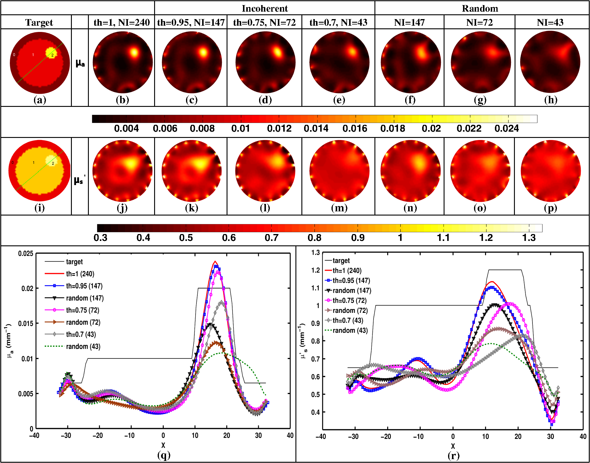
Once the indices (ind) are found, the corresponding phase components are also considered and only the incoherent measurements of the Jacobian ( $J$ ) and data-model misfit ( $δ$ ) are considered, given as

Eq. (9)

J_{i} = J (ind, :) and δ_{i} = δ (ind),

where

J_{i}

and

δ_{i}

represent the reduced Jacobian and data-model misfit, respectively and the dimension of

J_{i}

is

(2 * N I) \times (2 * N N)

, with

N I

being the number of incoherent/independent measurements. Now, the new update equation becomes

Eq. (10)

(Δ D^{i}, Δ μ_{a}^{i}) = J_{i}^{T} {{[J}_{i} J_{i}^{T} + λ I]}^{- 1} δ_{i}^{(i - 1)} .

It is important to note that the retained measurements in the reduced Jacobian ( $J_{i}$ ) and data-model misfit ( $δ_{i}$ ) correspond to a source–detector map, which indicates the highly influential source–detector configuration. As with the data-resolution matrix approach,¹¹ the ind were determined in the first iteration and utilized for subsequent iterations as there was no considerable variation in ind between the iterations.

4.3.

Estimating Regularization Parameter using Generalized Cross-Validation (GCV)

The proposed incoherence method to estimate the independent measurements were compared with a random-based measurement selection approach. In order to have an unbiased comparison between these methods, the GCV method was used to estimate the optimal regularization parameter ( $λ$ ) to compute the solution given by Eq. (10). The GCV method is a popular approach for estimating the regularization parameter ( $λ$ ) and this is obtained by minimizing a function $G (λ)$ defined as²¹

Eq. (11)

G (λ) = \frac{\sum_{k = 1}^{rank (J_{i})} {(\frac{u_{k}^{T} δ_{i}}{σ_{k}^{2} + λ^{2}})}^{2}}{{[\sum_{k = 1}^{rank (J_{i})} \frac{1}{σ_{k}^{2} + λ^{2}}]}^{2}} .

If $J_{i} {= U Σ V}^{T}$ represents the singular value decomposition of the Jacobian matrix then $u_{k}$ in the above equation denotes the $k$ ’th column of the matrix $U$ and $σ_{k}$ , the singular values of the Jacobian matrix. A computationally efficient simplex method is used to solve Eq. (11) to estimate the regularization parameter ( $λ$ ) and in turn this is used in Eq. (10) to estimate the optical properties for all the studies presented in this method. A detailed description of this method can be found in Ref. 21.

All computations were performed on a Linux workstation, which had 2.4 GHz Intel Quad core processor along with 8-GB RAM. The details of simulation and experimental studies performed as part of this work is presented in Sec. 5.

5. Simulation and Experimental Evaluation

5.1.

Numerical Experimental Data

For the simulation and experimental evaluation of the proposed method, the reconstruction problem was solved using nonlinear iterative method [Levenberg–Marquardt (LM) minimization scheme]. In order to show the dependency of regularization parameter ( $λ$ ) on the data resolution matrix, an irregular-shaped breast mesh was considered. Two finite element breast meshes were used, one for experimental data generation and another for reconstruction scheme. A fine mesh containing 4876 nodes with 9567 triangular elements was used for experimental data generation purpose, and for the reconstruction scheme a coarser mesh with 1969 nodes with 3753 triangular elements was considered. The background optical properties of the breast mesh were $μ_{a} = 0.01 {mm}^{- 1}$ and $μ_{s}^{'} = 1 {mm}^{- 1}$ . The target distribution mimicking a tumor had the following optical properties, $μ_{a} = 0.02 {mm}^{- 1}$ and $μ_{s}^{'} = 2 {mm}^{- 1}$ and was placed at $x = 20 mm$ and $y = 0 mm$ having a radius of 10 mm. The data collection setup had 16 fibers arranged in an equispaced fashion along the boundary of the imaging domain, where, when one fiber acted as a source, rest acted as detectors, resulting in 240 ( $16 \times 15$ ) measurement points.¹⁴ The source was positioned at one mean transport length inside the boundary and were modeled as having a Gaussian profile with full width half maximum (FWHM) of 3 mm to mimic the experimental conditions.¹⁴ The numerically generated data had 1% Gaussian noise to replicate the experimental case. The target distribution ( $μ_{a}$ and $μ_{s}^{'}$ ) for this case is shown in Figs. 1(a) and 1(h) labeled as “Target.”

Fig. 1

An example case showing the dependence of data-resolution matrix on regularization parameter ( $λ$ ) for independent measurement selection. The target distributions of $μ_{a}$ and $μ_{s}^{'}$ is given in (a) and (h), respectively. Panels (b)–(d) and (i)–(k) show the reconstructed distributions of $μ_{a}$ and $μ_{s}^{'}$ , respectively, using all measurements ( $N M = 240$ ) for a given $λ$ (indicated on top of each distribution). Panels (e)–(g) and (l)–(n) show the reconstructed results obtained using independent measurements selected via data-resolution matrix approach. The minimum, mean, and maximum value of the diagonal of the Hessian were the three choices of $λ$ (indicated on the top of each image).

In order to effectively assess the proposed technique in terms of determining the independent measurements based on incoherence, a numerical experiment with the same breast mesh and optical properties as described earlier was considered. The target distribution ( $μ_{a}$ and $μ_{s}^{'}$ ) for this case is shown in Figs. 2(a) and 2(i) labeled as “Target.” To evaluate the performance of the proposed method with complex shaped inclusions (targets), a rectangular-shaped target with $length = 16 mm$ and $breadth = 6 mm$ was placed at $x = - 15$ and $y = 0$ and a diffused tumor with $radius = 6.5 mm$ was placed at $x = 18$ and $y = 0$ . The optical properties of these targets and the noise level in the data remained the same as described earlier. The target distribution ( $μ_{a}$ and $μ_{s}^{'}$ ) for this case is shown in Figs. 3(a) and 3(g) labeled as “Target.”

Fig. 2

Reconstructed $μ_{a}$ and $μ_{s}^{'}$ distributions using incoherent and random-based measurement selection with 1% data noise level. Panels (a) and (i) correspond to $μ_{a}$ and $μ_{s}^{'}$ target distributions and (b) and (j) show the reconstructed distributions using all measurements (NI = 240). Panels (c)–(e) and (k)–(m) correspond to the reconstructed distributions obtained for incoherent measurement selection and similarly panels (f)–(h) and (n)–(p) correspond to random-based measurement selection, the number of measurements (NM) (and corresponding threshold (th) for incoherence-based selection) being indicated above each reconstructed image. (q) and (r): The one-dimensional (1-D) cross-sectional plots along the dashed line in (a) and (i) for various reconstructed images.

Fig. 3

(a)–(l) Similar effort as Fig. 2 except for two complex targets (rectangular and diffusive). (m) and (n) The 1-D cross-sectional plot along the dashed line given in the target image [(a) and (g)] for various reconstructed images presented.

As a third numerical experiment, the proposed method was tested on a reflection-mode configuration. A rectangular mesh with $width = 80 mm$ and $breadth = 40 mm$ was considered. A fine mesh containing 4981 nodes with 9088 triangular elements was used for experimental data generation purpose and a coarser mesh containing 3321 nodes with 6400 triangular elements was used for the reconstruction scheme. The data collection setup had 13 fibers arranged in an equispaced fashion along the boundary of the imaging domain (i.e., along $y = 20$ ) resulting in 169 ( $13 \times 13$ ) measurement points¹⁴ to mimic the reflection mode imaging setup. The source was positioned at one mean transport length inside the boundary and were modeled as having a Gaussian profile with FWHM of 3 mm to mimic the experimental conditions.¹⁴ The background optical properties of the rectangular mesh were $μ_{a} = 0.01 {mm}^{- 1}$ and $μ_{s}^{'} = 1 {mm}^{- 1}$ . The target distribution mimicking an absorption site had the following optical properties, $μ_{a} = 0.02 {mm}^{- 1}$ and $μ_{s}^{'} = 2 {mm}^{- 1}$ and was placed at $x = 2 mm$ and $y = 7 mm$ having a radius of 4.5 mm. The numerically generated data had 1% Gaussian noise to replicate the experimental case. The target distribution ( $μ_{a}$ and $μ_{s}^{'}$ ) for this case is shown in Figs. 4(a) and 4(i) labeled as “Target.”

Fig. 4

(a) to (p) Similar effort as Fig. 2 except that the imaging geometry being rectangular and data acquisition being done in reflection mode. (q) and (r) The 1-D cross-sectional plot along the dashed line given in the target image [(a) and (i)] for various reconstructed images presented.

5.2.

Experimental Phantom Data

Finally to assess the capability of the proposed method, an experimental phantom data-set was considered. In this case, a multilayered gelatin phantom of diameter 86 mm and height 25 mm was fabricated with heated mixtures of water (80%), gelatin (20%), India Ink was used for absorption and for scattering, ${TiO}_{2}$ (titanium oxide powder) to obtain different optical properties. Three distinct layers of gelatin were constructed by repeatedly hardening gel solutions to contain different amounts of ink and ${TiO}_{2}$ for varying optical absorption and scattering, respectively.²²^,²³ To mimic a tumor, a cylindrical hole of diameter 16 mm and height 24 mm was filled with liquid. The region marked as “0” represents the fatty layer with $μ_{a} = 0.0065 {mm}^{- 1}$ and $μ_{s}^{'} = 0.65 {mm}^{- 1}$ . The region marked as “1” represents the fibro-glandular layer with $μ_{a} = 0.01 {mm}^{- 1}$ and $μ_{s}^{'} = 1.0 {mm}^{- 1}$ . Finally, the region marked as “2” represents the tumor region with $μ_{a} = 0.02 {mm}^{- 1}$ and $μ_{s}^{'} = 1.2 {mm}^{- 1}$ as the optical properties. These optical properties were chosen based on the reported values in the literature²⁴^,²⁵ for these regions. The 2-D cross section ( $μ_{a}$ and $μ_{s}^{'}$ ) of the phantom with three different regions labeled as “1,” “2,” and “3” is shown in Figs. 5(a) and 5(i).

Fig. 5

Similar effort as Fig. 2 except for the case of experimental gelatin phantom data case.

This data was calibrated using a reference homogenous phantom to obtain the initial guess for optical properties ( $μ_{a}$ , $μ_{s}^{'}$ ).²⁰ For the reconstruction, a mesh of 1785 nodes corresponding to 3418 linear triangular elements was used.

6. Results and Discussion

First, an illustration of dependence of data-resolution matrix-based choice of independent measurements on the regularization parameter ( $λ$ ) and the standard (Levenberg–Marquardt) method with a noise level of 1% in the simulated data was taken up and is shown in Fig. 1. Figures 1(a) and 1(h) correspond to the $μ_{a}$ and $μ_{s}^{'}$ target distribution, respectively. Figures 1(b)–1(d) and 1(i)–1(k) represent the standard reconstruction result (without any reduction in the number of measurements) obtained for $λ$ corresponding to the three different values namely the minimum, mean, and the maximum value of the diagonal elements of the Hessian ( ${JJ}^{T}$ ) matrix were considered. The corresponding $λ$ values are mentioned at the top of each reconstructed image. The reconstruction result obtained with the application of data-resolution-based independent measurement selection are correspondingly given in Figs. 1(e)–1(g) and 1(l)–1(n). The number of independent measurements (NI) and threshold value (th) are indicated along with the regularization parameter ( $λ$ ) at the top of each reconstructed distribution. The results of Fig. 1 indicate that the data-resolution–based method is sensitive to $λ$ in choosing the independent measurements. Note that the threshold (th) was kept constant ( $th = 0.9$ , similar to the threshold chosen in Ref. 11) across different $λ$ ’s to show the relation between $λ$ and the number of independent measurements (NI). As the number of independent measurements and reconstructed image quality varies with different choice of $λ$ in data-resolution-based approach, this approach is more prone to biased results and hence might not be the best method to provide high level of data-collection optimization. Also note that the automated optimal choice of $λ$ is not an easy task.²¹^,²⁶

To evaluate the performance of the proposed method, a fair comparison was made with randomly selected measurements using an irregular imaging domain (breast mesh) as discussed in Sec. 5. The reconstructed results obtained using measurements selected by the incoherence property for various thresholds (Algorithm 1), indicated by th, are given in Figs. 2(c)–2(e) and 2(k)–2(m). Similarly, Figs. 2(f)–2(h) and 2(n)–2(p) give the reconstruction results obtained by random selection of same number of measurements, indicated by NI, mentioned in the top-row. Note that the reconstruction result obtained using all measurements is given in Figs. 2(b) and 2(j) (corresponding to $th = 1$ and $N I = 240$ ). A one-dimensional (1-D) cross-sectional plot for the reconstructed distributions shown in Figs. 2(q) and 2(r) along the dashed line shown in the target image is given in Figs. 2(a) and 2(i). From the results, it is evident that the random selection of measurements provides inferior reconstructions compared with the proposed method of selection of independent measurements. Among the threshold values used, the result corresponding to $th = 0.9$ ( $N I = 118$ ) is identical to the result obtained using all measurements ( $N I = 240$ ). More importantly, these results also indicate the capability of the proposed method in terms of providing the high level of optimization required in terms of finding the independent measurements without compromising the reconstructed image quality.

A similar effort using the same mesh was made to demonstrate the ability of the proposed method to reconstruct complex-shaped inclusions such as a rectangular and diffused targets. The target distributions of these complex-shaped inclusions are given in Figs. 3(a) and 3(g). The corresponding reconstructed distributions using the incoherence and the random selection-based methods are shown in Figs. 3(c)–3(f) and 3(i)–3(l). Figures 3(b) and 3(h) represent the images obtained using all the measurements. The GCV method (Sec. 4.3) is deployed for all the cases for choosing $λ$ . From the reconstructed distributions and the 1-D cross-sectional plot reveal, the superior nature of the proposed method to identify the influential measurements using the proposed scheme.

As last part of the numerical experiment, a rectangular imaging domain with reflection-mode configuration was taken up. Note that in this case the sources and detectors were fixed at only one end of the mesh representing the reflection-based data-collection configuration. The target distributions of both $μ_{a}$ and $μ_{s}^{'}$ are shown in Figs. 4(a) and 4(i), respectively. The reconstructed images using all the measurements is shown in Figs. 4(b) and 4(j). The reconstructed distributions using the proposed scheme and the random-based measurement selection methods are given in Figs. 4(c)–4(h) and Figs. 4(k)–4(p). The reconstructed results along with the 1-D cross-sectional plot for the reconstructed distributions [Figs. 4(q) and 4(r)] reveal the efficacy of the proposed scheme even with a reflection mode configuration to identify the independent measurements as compared with random-based selection. Even in this case, the GCV method was deployed to obtain the corresponding regularization parameter ( $λ$ ).

Next, the reconstructed $μ_{a}$ and $μ_{s}^{'}$ distributions using the experimental phantom data are presented in Fig. 5, again the proposed method was compared with randomly selected measurements. The target distributions is as shown in Figs. 5(a) and 5(i). The reconstruction result obtained using all measurements, corresponding to $th = 1$ , is given in Figs. 5(b) and 5(j). The thresholds (th) of 0.95, 0.75, and 0.7 were used to select the incoherent measurements, which resulted in 147, 72, and 43 measurements, respectively, and the resulting reconstructed $μ_{a}$ and $μ_{s}^{'}$ images are shown in Figs. 5(c)–5(e) and 5(k)–5(m), respectively. The random selection of the same number of measurements resulted in reconstructed $μ_{a}$ and $μ_{s}^{'}$ images as shown in Figs. 5(f)–5(h) and Figs. 5(n)–5(p), respectively. A 1-D cross-sectional plot along the dashed line shown in the target images has also been plotted in Figs. 5(q) and 5(r) for various reconstructed images shown in Figs. 5(a)–5(p). It is evident from the results of Fig. 5 that the incoherence-based selection with threshold being 0.95 was able to provide the same kind of reconstruction as with usage of all measurements. It is important to note that for the random selection of same number of measurements ( $N I = 147$ ) corresponding to $th = 0.95$ resulted in a highly distorted target, thus indicating that the proposed method (incoherence-based selection) is capable of providing independent measurements. Note that, the optimal selection only enables the required sensitivity without compromising the reconstructed image quality with an added advantage of making the reconstruction process computationally efficient. The random selection enables the computational efficient part, but compromises the reconstructed image quality (the same is illustrated in all numerical and experimental cases shown here). The random selection that was chosen here was purely random, resulting in almost same image quality irrespective of the choice.

This study (Fig. 5) also shows the reliability of the presented method, where the layered tissue model is adapted, mimicking the inhomogenous background. The threshold for obtaining solution that is close to the one obtained by using all measurements in this case is 0.95, leading to number of required measurements as 147. The achievable optimization is in the same order even for the other cases presented in this work, making it evident that the proposed method provides the high-level information about the independent measurements.

Finally, a normalized mean square error (NMSE) was used as a figure of merit in order to determine a good criterion for choosing the value of threshold (th). The NMSE essentially measures the degree of similarity between two images. The NMSE is defined as²⁷

Eq. (12)

NMSE = \frac{MSE}{σ_{x_{true}}^{2}},

where

σ_{x_{true}}^{2}

denotes the variance of the true image (

x_{true}

) and MSE represents the mean square error between the true image (

x_{true}

) and the reconstructed image (

x_{recon}

), given by²⁷

Eq. (13)

MSE = \frac{1}{N} {‖ x_{true} - x_{recon} ‖}^{2},

here,

N

represents the length of the image. The NMSE for the various reconstructed images (Figs. 2–5) is presented in Table 1. Note that the notation, NMSE denotes the average quantity of NMSE (

μ_{a}

) and NMSE (

μ_{s}^{'}

) to ease the task of selecting an optimal threshold (th). For the simulation and experimental cases, the optimal threshold is chosen such that the obtained NMSE is within 5% of the original NMSE (using all measurements).

Table 1

The normalized mean square error (NMSE) of results presented in this work for varying thresholds (given in parenthesis of second column) along with the number of independent measurements (NI) with respect to the target image in each case. The corresponding random-based measurement selection NMSE is given in the last column.

Case	Incoherence based		Random based
Case	NI (th)	NMSE	NI	NMSE
Breast mesh (Fig. 2)	240 (1)	0.18349	—	—
	118 (0.9)	0.18357	118	0.21230
	71 (0.7)	0.19225	71	0.25166
	49 (0.61)	0.23579	49	0.44265
Breast mesh (Fig. 3)	240 (1)	0.45229	—	—
	150 (0.94)	0.45641	150	0.48490
	101 (0.9)	0.48919	101	0.56841
Rectangular mesh (Fig. 4)	169 (1)	0.49015	—	—
	104 (0.95)	0.49912	104	0.55058
	86 (0.9)	0.53257	86	0.58409
	52 (0.8)	0.60818	52	0.72009
Experimental phantom (Fig. 5)	240 (1)	2.24150	—	—
	147 (0.95)	2.32010	147	2.69570
	72 (0.75)	2.655215	72	2.73401
	43 (0.7)	2.71612	43	2.82175

To systematically study the effect of threshold (th) on the reconstructed $μ_{a}$ and $μ_{s}^{'}$ distributions, different threshold values and the resulting NMSE and independent measurements have been plotted in Fig. 6(a) for the case of experimental phantom (Fig. 5). Note that the NMSE ( $μ_{a}$ , $μ_{s}^{'}$ ) corresponding to $th = 1$ uses all measurements (240). The results show that the NMSE increases with decreasing threshold and an optimal value exists, which provide the reconstructed image quality being same as with the usage of all measurements. For all the cases discussed in this work, the optimal threshold value is 0.9 or above as the NMSE is within 5% with respect to the image obtained using all the measurements.

Fig. 6

(a) NMSE [Eq. (12)] for both $μ_{a}$ and $μ_{s}^{'}$ for quantitatively selecting the optimal threshold in the experimental phantom case (Fig. 5) using varying thresholds (th) corresponding to independent measurements (indicated on the top) with respect to the target image. (b): The computation time (in seconds) for varying thresholds (th) and the corresponding independent measurements for each threshold is indicated above each bar.

In order to show the computational advantage of the proposed method, Fig. 6(b) shows the computation time for the results presented in Fig. 5 with varying values of threshold (th) from 0.1 through 1 in steps of 0.05. The $x$ -axis corresponds to the varying values of thresholds and correspondingly the $y$ -axis denotes the computational time in time (in seconds) to reconstruct the image, which includes calculating the Jacobian, overhead-time for estimating the incoherent measurements and estimating the regularization parameter until the data-model misfit ( ${‖ δ ‖}^{2}$ ) did not improve by more than 2% when compared with previous iteration. The number of measurements corresponding to each threshold is also mentioned above each bar.

A key contribution of this work is the establishment of a procedure to identify the influential/incoherent measurements. Such procedure is highly desirable in cases where the measurement set-up is expensive there by enabling to reduce the cost involved in the measurement set-up, other than the obvious computational time reduction [Fig. 6(b)]. One of the potential uses of the proposed method is in the case of dynamic diffuse optical imaging,¹²^,¹³ where the measurement time (increasing the frame-rate) and the cost of the set-up can be reduced by reducing the number of sources and detectors.

7. Conclusions

The image reconstruction problem in the diffuse optical imaging is typically rank-deficient, indicating that all the measurements do not provide the independent information. Determining the independent measurements among the available measurements is extremely beneficial in terms of faster data-collection and instrumentation associated with it. In this work, we have proposed a simple, yet novel, efficient method that can provide the specific information about particular measurement being independent or not, using the incoherence property of the sensitivity matrix. The proposed method was also shown to overcome the inherent limitation of regularization parameter dependency in choosing the independent measurements selection using the existing state of the art, data-resolution-based approach. The proposed method was validated to estimate both optical absorption and scattering coefficients using irregular-shaped (breast), rectangular (reflection-mode) imaging domain cases, and experimental gelatin phantom case. The corresponding computer code is made available as open-source for the usage of biomedical optical imaging community.²⁸

Acknowledgments

This work is supported by the Department of Biotechnology (DBT) Rapid Grant for Young investigators (RGYI) (No: BT/PR6494/GBD/27/415/2012).

References

1.

D. A. Boaset al., “Imaging the body with diffuse optical tomography,” IEEE Signal Process. Mag., 18 (6), 57 –75 (2001). http://dx.doi.org/10.1109/79.962278 ISPRE6 1053-5888 Google Scholar

2.

S. Srinivasanet al., “Interpreting hemoglobin and water concentration, oxygen saturation and scattering measured in vivo by near-infrared breast tomography,” Proc. Nat. Acad. Sci. U.S.A., 100 (21), 12349 –12354 (2003). http://dx.doi.org/10.1073/pnas.2032822100 PNASA6 0027-8424 Google Scholar

3.

J. C. Hebdenet al., “Three-dimensional optical tomography of the premature infant brain,” Phys. Med. Biol., 47 (23), 4155 –4166 (2002). http://dx.doi.org/10.1088/0031-9155/47/23/303 PHMBA7 0031-9155 Google Scholar

4.

S. R. ArridgeJ. C. Schotland, “Optical tomography: forward and inverse problems,” Inverse Probl., 25 (12), 123010 –123069 (2009). http://dx.doi.org/10.1088/0266-5611/25/12/123010 INPEEY 0266-5611 Google Scholar

5.

A. GibsonH. Dehghani, “Diffuse optical imaging,” Philos. Trans. R. Soc. A, 367 (1900), 3055 –3072 (2009). http://dx.doi.org/10.1098/rsta.2009.0080 PTRMAD 1364-503X Google Scholar

6.

J. P. Culveret al., “Optimization of optode arrangements for diffuse optical tomography: a singular-value analysis,” Opt. Lett., 26 (10), 701 –703 (2001). http://dx.doi.org/10.1364/OL.26.000701 APOPAI 0003-6935 Google Scholar

7.

P. K. Yalavarthyet al., “Experimental investigation of perturbation Monte-Carlo based derivative estimation for imaging low-scattering tissue,” Opt. Express, 13 (3), 985 –997 (2005). http://dx.doi.org/10.1364/OPEX.13.000985 OPEXFF 1094-4087 Google Scholar

8.

F. LeblondK. M. TichauerB. W. Pogue, “Singular value decomposition metrics show limitations of detector design in diffuse fluorescence tomography,” Biomed. Opt. Express, 1 (5), 1514 –1531 (2010). http://dx.doi.org/10.1364/BOE.1.001514 BOEICL 2156-7085 Google Scholar

9.

L. ChenN. Chen, “Optimization of source and detector configurations based on Cramer-Rao lower bound analysis,” J. Biomed. Opt., 16 (3), 035001 (2011). http://dx.doi.org/10.1117/1.3549738 JBOPFO 1083-3668 Google Scholar

10.

J. PrakashP. K. Yalavarthy, “Data-resolution based optimal choice of minimum required measurements for image-guided diffuse optical tomography,” Opt. Lett., 38 (2), 88 –90 (2013). http://dx.doi.org/10.1364/OL.38.000088 OPLEDP 0146-9592 Google Scholar

11.

D. KarkalaP. K. Yalavarthy, “Data-resolution based optimization of the data-collection strategy for near infrared diffuse optical tomography,” Med. Phys., 39 (8), 4715 –4725 (2012). http://dx.doi.org/10.1118/1.4736820 MPHYA6 0094-2405 Google Scholar

12.

C. B. ShawP. K. Yalavarthy, “Effective contrast recovery in rapid dynamic near-infrared diffuse optical tomography using

ℓ_{1}

-norm-based linear image reconstruction method,” J. Biomed. Opt., 17 (8), 086009 (2012). http://dx.doi.org/10.1117/1.JBO.17.8.086009 JBOPFO 1083-3668 Google Scholar

13.

S. Guptaet al., “Singular value decomposition based computationally efficient algorithm for rapid dynamic near-infrared diffuse optical tomography,” Med. Phys., 36 (12), 5559 –5567 (2009). http://dx.doi.org/10.1118/1.3261029 MPHYA6 0094-2405 Google Scholar

14.

T. O. McBrideet al., “Development and calibration of a parallel modulated near- infrared tomography system for hemoglobin imaging in vivo,” Rev. Sci. Instrum., 72 (3), 1817 –1824 (2001). http://dx.doi.org/10.1063/1.1344180 RSINAK 0034-6748 Google Scholar

15.

E. CandesM. Wakin, “An introduction to compressive sampling,” IEEE Signal Process. Mag., 25 21 –30 (2008). http://dx.doi.org/10.1109/MSP.2007.914731 ISPRE6 1053-5888 Google Scholar

16.

H. Dehghaniet al., “Near infrared optical tomography using NIRFAST: algorithms for numerical model and image reconstruction algorithms,” Commun. Numer. Methods Eng., 25 (6), 711 –732 (2009). http://dx.doi.org/10.1002/cnm.v25:6 CANMER 0748-8025 Google Scholar

17.

H. Dehghaniet al., “Numerical modelling and image reconstruction in diffuse optical tomography,” Philos. Trans. R. Soc. A, 367 (1900), 3073 –3093 (2009). http://dx.doi.org/10.1098/rsta.2009.0090 PTRMAD 1364-503X Google Scholar

18.

P. K. Yalavarthyet al., “Weight-matrix structured regularization provides optimal generalized least-squares estimate in diffuse optical tomography,” Med. Phys., 34 (6), 2085 –2098 (2007). http://dx.doi.org/10.1118/1.2733803 MPHYA6 0094-2405 Google Scholar

19.

A. Jinet al., “Preconditioning of the fluorescence diffuse optical tomography sensing matrix based on compressive sensing,” Opt. Lett., 37 (20), 4326 –4328 (2012). http://dx.doi.org/10.1364/OL.37.004326 OPLEDP 0146-9592 Google Scholar

20.

B. W. Pogueet al., “Calibration of near-infrared frequency-domain tissue spectroscopy for absolute absorption coefficient quantitation in neonatal head-simulating phantoms,” J. Biomed. Opt., 5 (2), 185 –193 (2000). http://dx.doi.org/10.1117/1.429985 JBOPFO 1083-3668 Google Scholar

21.

R. P. K. JagannathP. K. Yalavarthy, “Minimal residual method provides optimal regularization parameter for diffuse optical tomography,” J. Biomed. Opt., 17 (10), 106015 (2012). http://dx.doi.org/10.1117/1.JBO.17.10.106015 JBOPFO 1083-3668 Google Scholar

22.

B. W. PogueM. S. Patterson, “Review of tissue simulating phantoms for optical spectroscopy, imaging and dosimetry,” J. Biomed. Opt., 11 (4), 041102 (2006). http://dx.doi.org/10.1117/1.2335429 JBOPFO 1083-3668 Google Scholar

23.

P. K. Yalavarthyet al., “Structural information within regularization matrices improves near infrared diffuse optical tomography,” Opt. Express, 15 (13), 8043 –8058 (2007). http://dx.doi.org/10.1364/OE.15.008043 OPEXFF 1094-4087 Google Scholar

24.

B. Brooksbyet al., “Magnetic resonance guided near infrared tomography of the breast,” Rev. Sci. Instrum., 75 (12), 5262 –5270 (2004). http://dx.doi.org/10.1063/1.1819634 RSINAK 0034-6748 Google Scholar

25.

T. Durduranet al., “Bulk optical properties of healthy female breast tissue,” Phys. Med. Biol., 47 (16), 2847 –2861 (2002). http://dx.doi.org/10.1088/0031-9155/47/16/302 PHMBA7 0031-9155 Google Scholar

26.

J. PrakashP. K. Yalavarthy, “A LSQR-type method provides a computationally efficient automated optimal choice of regularization parameter in diffuse optical tomography,” Med. Phys., 40 (3), 033101 (2013). http://dx.doi.org/10.1118/1.4792459 MPHYA6 0094-2405 Google Scholar

27.

O. Elbadawyet al., “An information theoretic image-quality measure,” in IEEE Can. Conf. Electrical Comput. Eng., 169 –172 (1998). Google Scholar

28.

C. B. ShawP. K. Yalavarthy, “Incoherence based optimal selection of independent measurements in diffuse optical tomography,” (2013) https://sites.google.com/site/sercmig/home/incoherence September ). 2013). Google Scholar

Biography

Calvin B. Shaw received the BE degree from the M. S. Ramaiah Institute of Technology (MSRIT), Bangalore, India, in 2009, and the MSc [Engg.] degree from the Indian Institute of Science (IISc), Bangalore, India, in September 2012, in the Supercomputer Education and Research Centre (SERC), where he is currently working towards the PhD degree in medical imaging. His research interests include biomedical optical imaging, compressive sensing, sparse recovery methods, and inverse problems in medical imaging.

Phaneendra K. Yalavarthy received the MSc degree in engineering from the Indian Institute of Science, Bangalore, India, and the PhD degree in biomedical computation from Dartmouth College, Hanover, New Hampshire, in 2007. He is an assistant professor in the Supercomputer Education and Research Centre, the Indian Institute of Science, Bangalore. His research interests include medical image computing, medical image analysis, and biomedical optics.

Citation Download Citation

Calvin B. Shaw and Phaneendra K. Yalavarthy "Incoherence-based optimal selection of independent measurements in diffuse optical tomography," Journal of Biomedical Optics 19(3), 036017 (21 March 2014). https://doi.org/10.1117/1.JBO.19.3.036017

Published: 21 March 2014

Access the abstract

JOURNAL ARTICLE
11 PAGES

DOWNLOAD PAPER SAVE TO MY LIBRARY

GET CITATION

CITATIONS

Cited by 3 scholarly publications.

Explore citations on Lens.org

RIGHTS & PERMISSIONS

Get copyright permission Get copyright permission on Copyright Marketplace

KEYWORDS

Optical properties

Diffuse optical tomography

Absorption

Data modeling

Near infrared

Breast

Tissue optics

1.

Introduction

2.

NIR Diffuse Optical Tomography: Forward Problem

Eq. (1)

3.

NIR Diffuse Optical Tomography: Inverse Problem

Eq. (2)

Eq. (3)

Eq. (4)

4.

Independent Measurements Selection

4.1.

Data-Resolution Matrix-Based Approach

Eq. (5)

4.2.

Incoherence-Based Measurement Selection

Eq. (6)

Eq. (7)

Eq. (8)

Algorithm 1

Eq. (9)

Eq. (10)

4.3.

Estimating Regularization Parameter using Generalized Cross-Validation (GCV)

Eq. (11)

5.

Simulation and Experimental Evaluation

5.1.

Numerical Experimental Data

Fig. 1

Fig. 2

Fig. 3

Fig. 4

5.2.

Experimental Phantom Data

Fig. 5

6.

Results and Discussion

Eq. (12)

Eq. (13)

Table 1

Fig. 6

7.

Conclusions

Acknowledgments

References

Biography

Show All Keywords

Keywords/Phrases

Search In:

Publication Years