
|
|
1.IntroductionNoninvasive skin imaging is envisioned to play a prevalent role in the future of dermatology. Because of its accessibility, skin is amenable to noninvasive diagnostics and therapeutic monitoring; an additional important advantage offered by noninvasive skin imaging is timeliness, resulting in a more effective use of the clinician’s time spent treating a patient. Extensive research has been conducted in the past few decades toward developing noninvasive skin imaging and diagnostic modalities. Optical coherence tomography (OCT) offers the capability to image layers and structures well below the surface of the skin.1–5 Numerous studies using OCT have been performed to image subsurface layers and structures of skin, including the epidermis, dermal–epidermal junction, dermis, hair follicles, blood vessels, and sweat ducts.6–9 Clinical studies suggest that OCT may be useful for noninvasive diagnosis of skin diseases and to assess wound healing.2–5,10–17 The lateral resolution of conventional OCT instruments is limited to tens of micrometers, hampering the adoption of OCT in a wide range of applications that require cellular resolution comparable to or approaching histological resolution. The numerical aperture (NA) of the optics sets the lateral resolution in the focal plane of the optics and throughout the depth of focus. The depth of focus is inversely proportional to the NA. As a result, OCT typically operates at low NA of around 0.05 to 0.025 with a corresponding lateral resolution in the order of 10 to 20 μm, which enables a large depth of focus on the millimeter scale (0.6 to 2.4 mm). Various hardware and software methods have been investigated to address the trade-off between lateral resolution and depth of focus, including axicon lenses to generate Bessel beams or phase masks, holoscopy, and computational techniques. Bessel beams have successfully demonstrated imaging in biological tissue with lateral resolution ranging from to 8 μm, with extended depth of focus in the millimeter range.18–20 The main limitation of Bessel beams imaging has been the reduced light efficiency of these systems. Phase masks have been investigated to create an annular mask21 or add spherical aberration to the optical system,22 with a factor of to 3 improvement in the depth of focus at the expense of some loss of image quality throughout the range. Holoscopy, which combines full field Fourier-domain OCT and numerical reconstruction of digital holography, has been introduced as a solution to achieve extended depth of imaging with constant sensitivity and lateral resolution. The lateral resolution is not limited by the NA, but rather by the numerical reconstruction distance of the holograms. Depth of imaging of and lateral resolution of was reported.23 However, holoscopy suffers from noncompensated phase error caused by multiple scattering (nonballistic) photons in highly scattering samples.23 Computational methods such as three-dimensional (3-D) Fourier-domain resampling have been demonstrated in combination with interferometric synthetic aperture microscopy to extend the imaging depth to 1.2 mm in skin in vivo; these techniques require an accurate and stable phase measurement.24 Optical coherence microscopy (OCM) was introduced to achieve cellular resolution using a higher NA objective (i.e., ) than conventional OCT (i.e., ); the gain in resolution in OCM is reached at the expense of a limited depth of focus in the order of 100 to 200 μm.25 Gabor-domain optical coherence microscopy (GD-OCM) was proposed by our group in 2008 to dynamically extend the imaging depth of OCM26 and has since started to be adopted in other research groups as well.27 A liquid lens is dynamically refocused at different depth locations to acquire multiple images that are then combined in a single volume. The custom optics can refocus up to a 2-mm imaging depth. In skin, an imaging depth of about 0.6 mm was achieved with an invariant lateral resolution of 2 μm throughout the volume.28 Provided the increased lateral resolution by an order of magnitude compared with conventional OCT, the images acquired with GD-OCM have a shallower depth of focus around the focal plane controlled by the liquid lens, typically in the order of 60 to 100 μm.29 Therefore, in order to image a volume up to 0.6 mm in depth for example, the liquid lens is dynamically refocused six times to image six volumes, which are then fused in postprocessing to produce a volumetric image with 2-μm resolution throughout the 0.6-mm depth.30 The large dataset and the multiple computational tasks associated with GD-OCM compound the need for fast processing; performing the processing steps on conventional architectures takes about two orders of magnitude longer than the acquisition steps. Critical to the adoption of GD-OCM in the clinical workflow is a fast, real-time processing, and rendering of the high-resolution images. Recently, graphics processing units (GPUs) were shown to be powerful tools for general numerical simulation,31–35 signal processing,36 and image processing for a variety applications.37 The use of GPUs has been investigated for several imaging-related tasks, ranging from image processing steps to image-based modeling and clinical intervention guidance.38 The GPU technology was also reported to solve computational problems related to medical imaging.39,40 Several studies conducted in the last 4 years have shown how GPUs can improve the processing speed of OCT imaging.41–55 The use of multiple GPUs for OCT has also been investigated by peers. Huang et al.56 demonstrated the use of dual GPUs to simultaneously compute the structural image intensity and phase Doppler imaging of blood flow on both a phantom and the chorioallantoic membrane. The authors reported a frame rate of 70 fps with an image size of . The same authors demonstrated in a different paper GPU-based motion compensation of handheld manual scanning OCT.57 Zhang and Kang also investigated the use of dual GPUs architecture to speed up the processing and rendering steps of an OCT system designed to guide micromanipulation using a phantom model and vitreoretinal surgical forceps. The first GPU was dedicated to data processing, whereas the second was used for rendering and display. A volume rate of 5 volumes per second with the volume size of was reported.58 Later, the same group demonstrated the use of dual-GPU architecture to guide microsurgical procedures of microvascular anastomosis of the rat femoral artery and ultramicrovascular isolation of the retinal arterioles of the bovine retina.59 A display rate of 10 volumes per second for an image size of was reported. In these recent advancements with multiple GPUs, two GPUs were considered, where one GPU was typically dedicated to processing and another GPU was used for image rendering. Compared with OCT, GD-OCM faces additional challenges deriving from the higher imaging resolution of 2 μm that imposes 1-μm sampling, which results in a significantly larger dataset to be processed. Also, the computation and fusing of six volumes of data is a demanding task. We propose here a parallel computational framework using multiple GPUs to enable real-time imaging capabilities of GD-OCM. In the following sections, we review the architecture of the GD-OCM system and detail the imaging process in the central processing unit (CPU) in order to identify the computational bottleneck of the imaging process. We then describe the proposed parallelized GPU framework to overcome the limitations (See Sec. 3). 2.Methods2.1.System DescriptionThe current GD-OCM system fits on a movable cart. The handheld scanning probe is attached to an articulated arm that can be easily adjusted to fit the region of the skin that the clinician wants to image. The imaging system has micron-class resolution of 2 μm in skin tissue (average refractive index of 1.4), both axially and laterally. The light source is a superluminescent diode laser centered at 840 nm with 100 nm FWHM (BroadLighter D-840-HP-I, Superlum®, Ireland). The microscope objective probe with 2-mm field-of-view incorporates a liquid lens, which allows dynamic-focusing in order to image different depths of the sample while maintaining a lateral resolution of 2 μm within the imaging depth of up to by design.28,29 A custom dispersion compensator and a custom spectrometer with a high-speed CMOS line camera (spl4096-70 km, Basler Inc., Exton, Pennsylvania) are used to acquire the spectral information.60,61 With a set depth of focus of 100 μm, the liquid lens is refocused six times to image 600 μm in depth in skin tissue, yielding six volumes of data to acquire and to process. Conventionally, a skin sample of acquired with GD-OCM generates 49 GB (i.e., ) of data to be processed. Although the current total acquisition time is 1.43 min, the image processing steps on this high-resolution data may take up to 3.5 h on a conventional sequential architecture, as discussed in the following section, before the scanned data can be visualized in 3-D by a clinician. 2.2.Description of the Imaging Process in CPUThe imaging platform runs on a workstation equipped with a Supermicro X8DTG-QF motherboard. The system operates on 64 bit Microsoft® Windows® 7 with two processors Intel® core i7/Xeon (X5650 6-core 2.66-GHz CPUs, each with 12-MB cache) and 48 GB of RAM to allow the operating system to run smoothly while the GD-OCM images are being acquired. High-efficiency data security and storage on a 2.4-TB (eight Seagate 300GB SAS 15K hard drives) hard drive is made possible by an LSI, San Jose, California MegaRAID 9260 redundant array of independent disks (RAID) card. A Camera-link Bitflow frame grabber Karbon-CL, Woburn, Massachusetts is used to buffer the data from a camera, and a DAQ card (National Instruments, PCI-6733) is dedicated to control the galvanometer scanners and liquid lens and generate the trigger signal for the camera to synchronize the scanning and the acquisition at the beginning of each zone. In CPU-based processing, the imaging process consists of acquisition, postprocessing, fusing, and rendering steps. All these steps, excluding rendering, run on LabVIEW™ 2012 software (National Instruments, Austin, Texas). 2.2.1.AcquisitionThe acquisition step consists of lateral scanning of the same skin area six times with different focal lengths of the liquid lens. For each focal length, amplitude scans (A-scans) spectra with a lateral sampling interval of 1 μm are acquired. Data with single precision are saved in parallel on the hard drive in binary format. In order to run acquisition and saving independently, a buffer was created in LabVIEW™ to hold the acquired data while saving is in progress using the high-speed storage capability of RAID technology. After the acquisition of the first zone, the focal length is shifted to the next zone and the lateral scanning is repeated. After acquisition of all six zones, six A-scans are saved on the disk. The acquisition uses a high-speed CMOS line camera with , for an acquisition time of 14.3 μs per A-scan. The total acquisition time is then 1.43 min for the six zones. A further reduction in acquisition is anticipated with the higher frame rate cameras that have already reached the market. Each A-scan consists of a binary spectrum of 4096 pixels, thus the acquisition step generates 49 GB () of data that is saved to the disk for postprocessing. 2.2.2.PostprocessingAfter reading data from the disk, the postprocessing steps consist of performing DC removal, k-space linearization, fast-Fourier transform (FFT), gray scaling, and auto-synchronization. The DC term for each B-scan is a one-dimensional (1-D) array of 4096 pixels, which is obtained by computing the mean of the 1000 A-scans that form the B-scan. The DC term is then removed from each A-scan. Next, each A-scan undergoes k-space linearization, FFT, and gray level and log scaling using a modified version of existing functions in LabVIEW™. To achieve high-speed acquisition, the hardware synchronization is applied just once at the beginning of each zone. As a consequence, a drift in hardware synchronization between the camera and the scanning is experienced. An auto-synchronization software was developed and implemented to compensate the drift with an intercorrelation algorithm applied between two consecutive B-scans. The peak of the intercorrelation corresponds to the number of shifted A-scans. The region of interest of the shift-compensated frames is buffered in the memory for the fusing step. Each zone has a dedicated buffer to facilitate the fusing step. The total postprocessing time, including reading data, is 29 min for one zone, yielding 2.9 h for six zones (see detailed timing in Table 1). Table 1Timing of the processing steps and computational speed-up between sequential and pipelined implementations.
2.2.3.FusingIn the fusing step, the six zones of the sample are fused in one volume using the Gabor fusion technique.27,62 For each B-scan, the six frames are accessed from the buffers; only the focused region (the region within around the focal plane) of the six frames contributes to the final image. Thus, each frame is multiplied by a window of width centered at the focal plane of the dynamic focus probe. The window serves as a weighting function for each frame in the fusing process. The six windows are preoptimized based on the voltage applied to the liquid lens and the focal shift for each acquired image. The final image is obtained by adding the six windowed frames. All focused B-scan frames are saved back to the disk using binary format. The computation time for the fusing process is estimated at 20 min, accounting for the disk saving time. 2.2.4.RenderingVoxx and open source ImageJ are used to render the volumetric image and display the two-dimensional (2-D) and 3-D images. The time needed for rendering is . In summary, the 3-D imaging and visualization of a sample using a sequential implementation takes about 3.5 h. The analysis of the sequential implementation (Table 1) shows that the k-space linearization is the most time-consuming operation (44%); followed by the gray level and log scaling (29%); fusing (8%); DC removal (8%); FFT (7%). Saving, loading, and auto-synchronization account for 4% altogether. As a next step to increase the computational speed on CPU, the use of pipelined computation was investigated, in which the operations with independent parameters are regrouped in different operation blocks, leveraging more advanced multithread CPU capabilities. Specifically, a process pipelining approach was employed, in which different operation blocks in the postprocessing and fusing steps were separated and performed in a pipelined manner. Figure 1 shows the flowchart of the proposed pipelined computation architecture in which the two most time-consuming operations are separated in two different blocks running in parallel. In the first block, the input A-scan data are loaded into a queue data structure while they are also simultaneously accessed for image processing in the second operation block, which consists of three sequential steps—DC removal, k-space linearization, and FFT. Similarly, another queue data structure is used to hold the modulus of the FFT outputs. The last operation block, dedicated to log scaling, auto-synchronization, and fusing, accesses the queue in a parallel manner and saves the final fused data into the hard drive. Table 1 summarizes the computational speed-up of the pipelined approach as compared with the sequential implementation. The pipelined CPU implementation completes processing one zone in , offering a speed-up over the 32 min of the sequential implementation. In this computation, as in prior work, k-space linearization is the bottleneck. In prior investigations, hardware solutions to k-linearization have been reported with good results.63–65 However, regardless of the approach to addressing the bottleneck, real-time imaging on CPU cannot be achieved, even with the pipelined approach. The CPU implementation is fundamentally limited by the number of cores compared with GPU that can allow more advanced parallelization implementation for the entire processing. 2.3.Proposed Multi-GPU Framework for GD-OCMSince the 1-D A-scan signals can be processed independently of each other, a parallelized scalable processing can fully leverage a multi-GPU system. The multi-GPU framework was designed to achieve the acquisition of each zone in parallel with the processing of the previous zone and yields the 3-D visualization of the sample within seconds after the acquisition of the entire volume is completed. The motherboard of the workstation (Supermicro®) can hold up to four GPUs and was configured based on the requirement to complete the processing of one zone within seconds, while the next zone is being acquired. Each of the GPUs is connected to the main system using a PCIe-2.0 connectivity facilitating up to data transfers between the CPU and each of the GPUs. The GPU processes run independently of each other and can occasionally communicate with each other using the PCIe-2.0 connectivity, with the CPU forming the intermediary communication step. Buffers are used, as in the CPU implementation, to serve as temporary memory. After the processing of each frame, only the focused region () is held in the GPU buffer, thus dividing by six the size of data to be managed during the fusing step. Figure 2 shows a schematic of the GD-OCM instrument and the proposed architecture of the multi-GPU-based GD-OCM imaging system. The acquisition time for each of the six zones, accounting for the focal length of the liquid lens being adjusted six times, is 14.3 s. During the acquisition of the first zone, which consists of a data size of A-scans, the data is held in a temporary CPU buffer. When the acquisition of this zone is completed, the data is structured and divided into four sections, which are transferred to the four GPUs via the four PCIe-2.0 interfaces. During that time, the focal length of the liquid lens is shifted by 100 μm to acquire the next zone. The acquisition of the next zone is done in parallel with the processing of the previous zone. The processing consists of DC removal, k-space linearization, computer unified device architecture (CUDA) FFT, gray level and log scaling, and auto-synchronization. Once the processing is completed for each frame, the resultant data is windowed to retain only the focused region. Data is held in temporary buffers in each GPU to be fused with the next zone. The GPUs are then released to handle processing of the next available zone. After the processing of each zone, the focused region is fused with the previous fusing result and hold in GPU memory as illustrated in Fig. 3 for one B-scan (1000 A-scans). Once all six zones are processed, visualization of the 3-D scan is enabled by GPU-based volume rendering, as well as 2-D visualization. Visualizing the 3-D structure in real-time is a computationally complex task mainly because of the size of the 3-D data (). For this study, the rendering was performed with GPU-based real-time volume rendering in one of the GPUs, providing a rendering time of 50 ms for one volume. Fig. 2Multi-graphics processing unit (GPU) architecture for Gabor-domain optical coherence microscopy. The frame grabber is connected to the workstation’s motherboard (Supermicro®) using PCIe x8. Red color blocks represent the buffering steps. Large arrows represent data transfer of a batch of frames, whereas narrow arrows represent transfer of an individual frame. Double-direction arrows between image processing steps and fused data blocks illustrate the exchange of frames between these two steps. The feedback arrow (Zone # Loop) represents the release of GPUs to handle the next zone. Each of the four GPUs runs independently during the processing and fusing and communicates with the other GPUs during the rendering.  2.4.Implementation of the Multi-GPU FrameworkThe software development framework for the proposed system consists of LabVIEW™ 2012 and NVIDIA® CUDA 5.0 programming interfaces. LabVIEW™ was employed to interface with the GD-OCM image acquisition system and to control access to the GPU cards. Communication between LabVIEW™ and CUDA was achieved with a dynamic-link library (DLL) developed in Microsoft® Visual Studio 2010. The different steps of the processing, including DC removal, k-space linearization, gray scaling, and auto-synchronization, were implemented in C++ using Microsoft® Visual Studio 2010; CUDA Fast Fourier Transform (CUFFT) was performed with the existing function in the CUDA environment. Parallelized access to the GPUs was made possible via multiple DLL calls with parameters such as the GPU identity, calibration, and frame-related parameters. Although each DLL call was designed to employ multiple cores in parallel, a set of DLL calls was implemented in parallel to fully employ the GPU cores available in each GPU and initiate the GPU boost capability. 3.Results and Discussion3.1.Run-Time Analysis of the Multi-GPU FrameworkFor the run-time analysis, five system configurations were investigated, as reported in Table 2. Systems A and B consisted of two GTX 680s and two GTX Titans GPUs, respectively, both of which employ adaptive processor and memory overclocking. Systems C and D consisted of four NVIDIA® C1060 and C2050 general purpose GPUs, which did not employ adaptive processor and memory overclocking. System E employed an Intel core i7 processor, which provided the benchmark CPU performance. Table 2System configurations investigated for Gabor-domain optical coherence microscopy (GD-OCM) processing.
Table 3 presents the average cumulative run times for the different configurations of Table 2. The run times are presented for a single GPU and all GPU scenarios, processing a total of A-scans. It can be seen that, using System A, a computational time of 29 s with a single GPU and 13 s with two GPUs was obtained. System B provided an average performance of 31 s with a single GPU and 15 s with two GPUs. Compared with a pipelined CPU running time benchmarked at 19 min, Systems A and B produce a computational speed-up of and , respectively—close to two orders of magnitude speed up. Systems C and D, which employ four GPUs, provided an average computation time of 235 and 115 s, respectively. Their lower performance is attributed to a lower number of processing cores in the system. Table 3Computational results using the multi GPU-based GD-OCM image processing for a data volume of 1000×1000 A-scans.
Figure 4 presents the average cumulative run time results for the image processing using configurations A and B. For both systems, the performance of the GPUs improved as the number of parallel A-scans being processed was increased. The overall computation time decreased exponentially with an increase in the number of parallel A-scans. For the case in which a total of 8k A-scans were processed in parallel, System A provided an average computation time of 175 and for the one and two GPU setups, respectively, whereas System B provided computation times of 156 and 82 s. Fig. 4GPU boost comparison for Systems A and B as a function of the total number of A-scans processed in parallel.  The results show the scalability of the proposed framework, which is critical for the improvement of the computational speed. From Fig. 4, it can be observed that the computational time taken by two GPUs to perform a given number of A-scans in parallel is equal to around half the computation time taken by a single GPU to perform the same amount of A-scans. Such an observation supports the fact that the framework is agnostic to the number of GPUs used for the computation and thus provides a scalable computational time. In comparing Systems A and B, as the number of parallel A-scans is increased up to 40k, the performance of the two systems is quite comparable. The slight improvement in the performance of the GTX 680 compared with GTX Titan, which has almost twice the number of processing cores, can be attributed to the adaptive processor overclocking achieved by the GPU boost algorithm on the NVIDIA® GTX 680 cards.35 As the GD-OCM setup was limited by the camera acquisition time (14.3 s per zone), the number of parallel A-scans processing was set to 40k for System A to yield a processing time that was faster than the acquisition time. Nevertheless, the implementation presented here leads to a scalable real-time GD-OCM image processing with a finite increase in the number of GPUs used in computation. Table 4 shows the detailed processing time for one zone ( A-scans) on System A with 40k total parallel A-Scan calls per iteration. Table 4Computational speed-up of the multi GPU based GD-OCM image processing compared with a pipelined CPU implementation.
The parallelized two-GTX 680s configuration of System A provided a computational time of 13.64 s for one zone ( A-Scans), yielding a computational speed of . As compared with the pipelined CPU implementation, this gain corresponds to a computational speed-up of over one order of magnitude. The ability of the proposed framework to account for a larger number of parallel A-scans can be extrapolated from trends observed in Fig. 4; it can be seen that, based on the required computation time, the optimal number of A-scans to be processed in parallel can be selected. As multiple cards are being considered, thermal management of the cards is needed to avoid over-heating, which could lead to a failure of the system—an important consideration for use of the system in a clinical environment where a repeated usage for imaging the patient’s anatomy is needed. Instability was experienced on GPU performance when the temperature of the cards went over . This occurred when the number of parallel GPU calls was increased. Effective thermal dissipation design that optimally removes heat from all the GPUs, while maintaining the PCs form factor, is critical. As an example, new PC form factors with unified thermal dissipation mechanisms for effective heat removal in GPUs have been investigated by Apple Inc., Cupertino, California66 In addition, recent developments in NVIDIA GPUs (Tegra K1) have focused on using a significantly reduced power source while maintaining optimal performance as a means to address GPU over-heating.67 Although such designs are in their initial stages of development, future advancements in PC form factors and GPU designs will address the over-heating issue effectively. The proposed multi-GPU computational framework offers the opportunity to reduce the processing time by the optimal choice of number of parallelization and GPU cards while preserving long-term use of the system. Also, a fully integrated C++ interface is considered to optimize the overall system robustness. 3.2.Processing-Based Image Quality AnalysisThe image quality of CPU- and GPU-based processing of the same A-scan was investigated at different steps of the processing to ensure that the same algorithm was implemented on CPU and GPU. For each A-scan the output arrays of each step with CPU and GPU were compared; no difference was found. Figure 5 shows the 2-D image of the same B-scan processed on CPU and on GPU with neither visual nor statistical difference. Fig. 5Image comparison between CPU and GPU processing of the same B-scan (zone 3 before the fusing). (a) CPU-based image processing, (b) GPU-based image processing. The depths reported are the distances in skin tissue (). The GPU image was acquired with the architecture A (Two GTX 680). 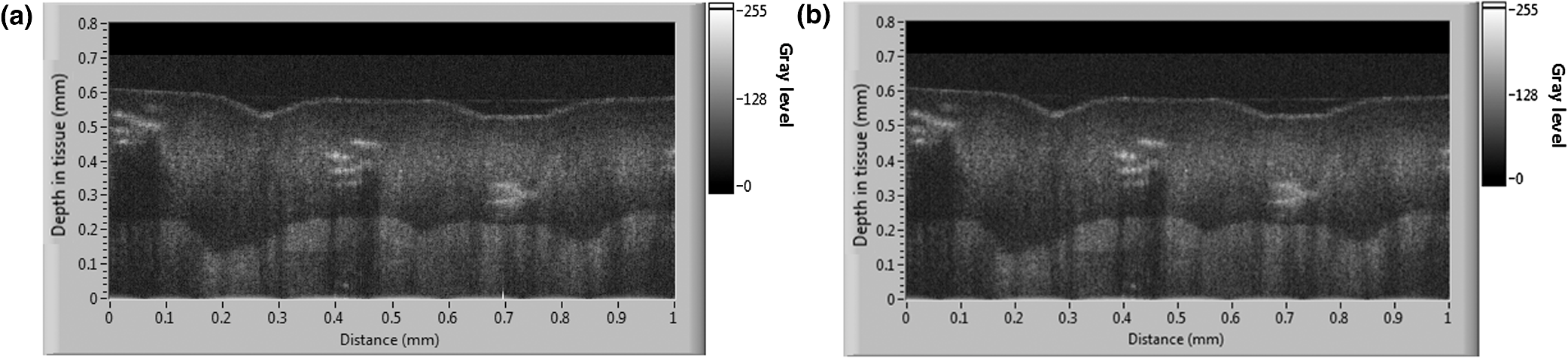 The proposed GPU framework was used to image the pointer fingertip. Figure 6 presents three orthogonal views as well as a 3-D volume of the processed and rendered volume using the proposed GPU framework. The cross sectional images of and planes [Figs. 6(a) and 6(c)] show the different layers of the skin (SC: stratum corneum, SG: stratum granulosum, SS: stratum spinosum, and SB: stratum basale). The en face images of plane [Figs. 6(d) and 6(e)] show the granulosum cells nuclei and blood vessels, respectively, demonstrating the high-lateral resolution of the imaging system. Figure 6(b) shows a snap shot of the 3-D volume of 1 mm by 1 mm by 0.6 mm rendered on GPU using max intensity renderer. Fig. 6GPU-based three-dimensional (3-D) image of the pointer fingertip acquired with the architecture A (Two GTX 680); (a) and (c) represent the cross sectional images of and planes and show the different layers of the skin (SC: stratum corneum, SG: stratum granulosum, SS: stratum spinosum, and SB: stratum basale); (d) and (e) show en face images of plane at two different depths; plane (d) at around the stratum granulosum layer shows the cells nuclei whereas blood vessels can be observed on the plane (e) just below the stratum basal; (b) snap shot of the 3-D volume of 1 mm by 1 mm by 0.6 mm shows the sweat ducts.  4.ConclusionA scalable and parallelized multi-GPU processing framework was proposed to overcome the processing speed limitation of GD-OCM. Five different scenarios of multi-GPU configurations were tested, and the use of two GTX 680 cards was found to yield the best performance for this application. For one zone (), an average performance of when processing 40k A-scans in parallel on both cards was achieved, yielding a processing speed of . This enables real-time processing of a skin volume of with 2-μm resolution. In particular, the goal of reducing the processing time to be faster than the acquisition time was achieved. Over one order of magnitude computational speed-up was obtained compared with the pipelined CPU processing, with no quantitative loss of image information. Importantly, results show that if two GPUs are considered the clinician can visualize the 3-D volume 13 s after the acquisition is completed, and that time is estimated at 6.5 s with four GPUs based on the demonstrated scalability of the framework. Thus, the proposed framework enables real-time processing, a fundamental step on the path toward adoption of GD-OCM in a clinical environment. AcknowledgmentsThis research was funded by the NYSTAR Foundation (C050070), NIH core grant in dermatology, NIH Training Grant EY007125, and the University of California, Los Angeles. Patrice Tankam would also like to thank the Center for Visual Science for his postdoctoral fellowship. We acknowledge NVIDIA® for the donation of two GeForce® GTX Titan GPUs to LighTopTech Corp. Competing financial interests: J. P. R. and C. C. are co-founders of LighTopTech Corp., which is licensing intellectual property from the University of Rochester related to Gabor Domain Optical Coherence Microscopy. Other authors declare no competing financial interests. ReferencesW. Drexleret al.,
“In vivo ultrahigh-resolution optical coherence tomography,”
Opt. Lett., 24
(17), 1221
–1223
(1999). http://dx.doi.org/10.1364/OL.24.001221 OPLEDP 0146-9592 Google Scholar
V. R. Kordeet al.,
“Using optical coherence tomography to evaluate skin sun damage and precancer,”
Lasers Surg. Med., 39
(9), 687
–695
(2007). http://dx.doi.org/10.1002/(ISSN)1096-9101 LSMEDI 0196-8092 Google Scholar
J. Welzelet al.,
“OCT in dermatology,”
Optical Coherence Tomography, 1103
–1122 Springer, Berlin, Heidelberg
(2008). Google Scholar
R. Pomerantzet al.,
“Optical coherence tomography used as a modality to delineate basal cell carcinoma prior to Mohs micrographic surgery,”
Case Rep. Dermatol., 3
(3), 212
–218
(2011). http://dx.doi.org/10.1159/000333000 Google Scholar
M. Mogensenet al.,
“OCT imaging of skin cancer and other dermatological diseases,”
J. Biophotonics, 2
(6–7), 442
–451
(2009). http://dx.doi.org/10.1002/jbio.v2:6/7 JBOIBX 1864-063X Google Scholar
F. G. Becharaet al.,
“Histomorphologic correlation with routine histology and optical coherence tomography,”
Skin Res. Technol., 10
(3), 169
–173
(2004). http://dx.doi.org/10.1111/j.1600-0846.2004.00038.x 0909-752X Google Scholar
M. C. Pierceet al.,
“Advances in optical coherence tomography imaging for dermatology,”
J. Invest. Dermatol., 123
(3), 458
–463
(2004). http://dx.doi.org/10.1111/jid.2004.123.issue-3 JIDEAE 0022-202X Google Scholar
R. SteinerK. Kunzi-RappK. Scharffetter-Kochanek,
“Optical coherence tomography: clinical applications in dermatology,”
Med. Laser Appl., 18
(3), 249
–259
(2003). http://dx.doi.org/10.1078/1615-1615-00107 1615-1615 Google Scholar
A. Alexet al.,
“Multispectral in vivo three-dimensional optical coherence tomography of human skin,”
J. Biomed. Opt., 15
(2), 026025
(2010). http://dx.doi.org/10.1117/1.3400665 JBOPFO 1083-3668 Google Scholar
L. E. Smithet al.,
“Evaluating the use of optical coherence tomography for the detection of epithelial cancers in vitro,”
J. Biomed. Opt., 16
(11), 116015
(2011). http://dx.doi.org/10.1117/1.3652708 JBOPFO 1083-3668 Google Scholar
B. J. Vakocet al.,
“Cancer imaging by optical coherence tomography—preclinical progress and clinical potential,”
Nat. Rev. Cancer, 12
(5), 363
–368
(2012). http://dx.doi.org/10.1038/nrc3235 NRCAC4 1474-175X Google Scholar
R. Wesselset al.,
“Optical biopsy of epithelial cancers by optical coherence tomography (OCT),”
Lasers Med. Sci., 1
–9
(2013). Google Scholar
J. M. Olmedoet al.,
“Correlation of thickness of basal cell carcinoma by optical coherence tomography in vivo and routine histologic findings: a pilot study,”
Dermatol. Surg., 33
(4), 421
–426
(2007). http://dx.doi.org/10.1111/dsu.2007.33.issue-4 DESUFE 1076-0512 Google Scholar
T. Gambichleret al.,
“In vivo optical coherence tomography of basal cell carcinoma,”
J. Dermatol. Sci., 45
(3), 167
–173
(2007). http://dx.doi.org/10.1016/j.jdermsci.2006.11.012 JDSCEI 0923-1811 Google Scholar
P. Wilder-Smithet al.,
“Noninvasive imaging of oral premalignancy and malignancy,”
J. Biomed. Opt., 10
(5), 051601
(2005). http://dx.doi.org/10.1117/1.2098930 JBOPFO 1083-3668 Google Scholar
W. B. Armstronget al.,
“Optical coherence tomography of laryngeal cancer,”
The Laryngoscope, 116
(7), 1107
–1113
(2006). http://dx.doi.org/10.1097/01.mlg.0000217539.27432.5a LARYA8 0023-852X Google Scholar
T. Hinzet al.,
“Preoperative characterization of basal cell carcinoma comparing tumour thickness measurement by optical coherence tomography 20-MHz ultrasound and histopathology,”
Acta Derm. Venereol., 92
(2), 132
–137
(2012). http://dx.doi.org/10.2340/00015555-1231 ADVEA4 0001-5555 Google Scholar
Z. Dinget al.,
“High-resolution optical coherence tomography over a large depth range with an axicon lens,”
Opt. Lett., 27
(4), 243
–245
(2002). http://dx.doi.org/10.1364/OL.27.000243 OPLEDP 0146-9592 Google Scholar
K.-S. LeeJ. P. Rolland,
“Bessel beam spectral-domain high-resolution optical coherence tomography with micro-optic axicon providing extended focusing range,”
Opt. Lett., 33
(15), 1696
–1698
(2008). http://dx.doi.org/10.1364/OL.33.001696 OPLEDP 0146-9592 Google Scholar
C. Blatteret al.,
“Extended focus high-speed swept source OCT with self-reconstructive illumination,”
Opt. Express, 19
(13), 12141
–12155
(2011). http://dx.doi.org/10.1364/OE.19.012141 OPEXFF 1094-4087 Google Scholar
A. Zlotniket al.,
“Improved extended depth of focus full field spectral domain Optical Coherence Tomography,”
Opt. Commun., 283
(24), 4963
–4968
(2010). http://dx.doi.org/10.1016/j.optcom.2010.07.053 OPCOB8 0030-4018 Google Scholar
K. Sasakiet al.,
“Extended depth of focus adaptive optics spectral domain optical coherence tomography,”
Biomed. Opt. Express, 3
(10), 2353
–2370
(2012). http://dx.doi.org/10.1364/BOE.3.002353 BOEICL 2156-7085 Google Scholar
D. Hillmannet al.,
“Holoscopy—holographic optical coherence tomography,”
Opt. Lett., 36
(13), 2390
–2392
(2011). http://dx.doi.org/10.1364/OL.36.002390 OPLEDP 0146-9592 Google Scholar
A. Ahmadet al.,
“Real-time in vivo computed optical interferometric tomography,”
Nat. Photonics, 7 444
–448
(2013). http://dx.doi.org/10.1038/nphoton.2013.71 1749-4885 Google Scholar
A. D. Aguirreet al.,
“High-resolution optical coherence microscopy for high-speed,”
Opt. Lett., 28
(21), 2064
–2066
(2003). http://dx.doi.org/10.1364/OL.28.002064 OPLEDP 0146-9592 Google Scholar
J. P. Rollandet al.,
“Gabor domain optical coherence microscopy,”
Proc. SPIE, 7139 71390F
(2008). http://dx.doi.org/10.1117/12.816930 PSISDG 0277-786X Google Scholar
P. BouchalA. BraduA. G. Podoleanu,
“Gabor fusion technique in a Talbot bands optical coherence tomography system,”
Opt. Express, 20
(5), 5368
–5383
(2012). http://dx.doi.org/10.1364/OE.20.005368 OPEXFF 1094-4087 Google Scholar
S. MuraliK. P. ThompsonJ. P. Rolland,
“Three-dimensional adaptive microscopy using embedded liquid lens,”
Opt. Lett., 34
(2), 145
–147
(2009). http://dx.doi.org/10.1364/OL.34.000145 OPLEDP 0146-9592 Google Scholar
S. Muraliet al.,
“Assessment of a liquid lens enabled in vivo optical coherence microscope,”
Appl. Opt., 49
(16), D145
–D156
(2010). http://dx.doi.org/10.1364/AO.49.00D145 APOPAI 0003-6935 Google Scholar
K.-S. Leeet al.,
“Cellular resolution optical coherence microscopy with high acquisition speed for in-vivo human skin volumetric imaging,”
Opt. Lett., 36
(12), 2221
–2223
(2011). http://dx.doi.org/10.1364/OL.36.002221 OPLEDP 0146-9592 Google Scholar
A. W. Greynolds,
“Multi-core and GPU accelerated simulation of a radial star target imaged with equivalent t-number circular and Gaussian pupils,”
Proc. SPIE, 8841 88410F
(2013). http://dx.doi.org/10.1117/12.2021036 PSISDG 0277-786X Google Scholar
J. Bolzet al.,
“Sparse matrix solvers on the GPU: conjugate gradients and multigrid,”
ACM Trans. Graphics, 22
(3), 917
–924
(2003). http://dx.doi.org/10.1145/882262 ATGRDF 0730-0301 Google Scholar
C. J. ThompsonH. SahngyunM. Oskin,
“Using modern graphics architectures for general-purpose computing: a framework and analysis,”
in Proc. 35th Ann. IEEE/ACM Int. Symp. Microarchitect. (MICRO-35),
(2002). Google Scholar
J. KrügerR. Westermann,
“Linear algebra operators for GPU implementation of numerical algorithms,”
ACM Trans. Graphics, 22
(3), 908
–916
(2003). http://dx.doi.org/10.1145/882262 ATGRDF 0730-0301 Google Scholar
R. Fernando, GPU Gems: Programming Techniques, Tips and Tricks for Real-Time Graphics, Addison-Wesley Professional, Indianapolis, Indiana
(2004). Google Scholar
V. M. Boveet al.,
“Real-time holographic video images with commodity PC hardware,”
Proc. SPIE, 5664 255
–262
(2005). http://dx.doi.org/10.1117/12.585888 Google Scholar
N. Masudaet al.,
“Computer generated holography using a graphics processing unit,”
Opt. Express, 14
(2), 603
–608
(2006). http://dx.doi.org/10.1364/OPEX.14.000603 OPEXFF 1094-4087 Google Scholar
A. P. Santhanamet al.,
“A multi-GPU real-time dose simulation software framework for lung radiotherapy,”
Int. J. Comput. Assisted Radiol. Surg., 7
(5), 705
–719
(2012). http://dx.doi.org/10.1007/s11548-012-0672-y Google Scholar
Y. Minet al.,
“A GPU-based framework for modeling real-time 3D lung tumor conformal dosimetry with subject-specific lung tumor motion,”
Phys. Med. Biol., 55 5137
–5149
(2010). http://dx.doi.org/10.1088/0031-9155/55/17/016 PHMBA7 0031-9155 Google Scholar
A. Santhanamet al.,
“Effect of 4D-CT image artifacts on the 3D lung registration accuracy: a parametric study using a GPU-accelerated multi-resolution multi-level optical flow,”
J. Med. Phys., 40
(6), SU-E-J-73
(2013). http://dx.doi.org/10.1118/1.4814285 0971-6203 Google Scholar
Y. Watanabeet al.,
“Real-time processing for full-range Fourier-domain optical-coherence tomography with zero-filling interpolation using multiple graphic processing units,”
Appl. Opt., 49
(25), 4756
–4762
(2010). http://dx.doi.org/10.1364/AO.49.004756 APOPAI 0003-6935 Google Scholar
K. ZhangJ. U. Kang,
“Graphics processing unit accelerated non-uniform fast Fourier transform for ultrahigh-speed, real-time Fourier-domain OCT,”
Opt. Express, 18
(22), 23472
–23487
(2010). http://dx.doi.org/10.1364/OE.18.023472 OPEXFF 1094-4087 Google Scholar
U.-S. Junget al.,
“Simple spectral calibration method and its application using an index array for swept source optical coherence tomography,”
J. Opt. Soc. Korea, 15
(4), 386
–393
(2011). http://dx.doi.org/10.3807/JOSK.2011.15.4.386 1226-4776 Google Scholar
K. ZhangJ. U. Kang,
“Real-time numerical dispersion compensation using graphics processing unit for Fourier-domain optical coherence tomography,”
Electron. Lett., 47
(5), 309
–310
(2011). http://dx.doi.org/10.1049/el.2011.0065 ELLEAK 0013-5194 Google Scholar
Y. JianK. WongM. V. Sarunic,
“Graphics processing unit accelerated optical coherence tomography processing at megahertz axial scan rate and high resolution video rate volumetric rendering,”
J. Biomed. Opt., 18
(2), 026002
(2013). http://dx.doi.org/10.1117/1.JBO.18.2.026002 JBOPFO 1083-3668 Google Scholar
M. Sylwestrzaket al.,
“Four-dimensional structural and Doppler optical coherence tomography imaging on graphics processing units,”
J. Biomed. Opt., 17
(10), 100502
(2012). http://dx.doi.org/10.1117/1.JBO.17.10.100502 JBOPFO 1083-3668 Google Scholar
N. H. Choet al.,
“High speed SD-OCT system using GPU accelerated mode for in vivo human eye imaging,”
J. Opt. Soc. Korea, 17
(1), 68
–72
(2013). http://dx.doi.org/10.3807/JOSK.2013.17.1.068 1226-4776 Google Scholar
Y. HuangJ. U. Kang,
“Real-time reference A-line subtraction and saturation artifact removal using graphics processing unit for high-frame-rate Fourier-domain optical coherence tomography video imaging,”
Opt. Eng., 51
(7), 073203
(2012). http://dx.doi.org/10.1117/1.OE.51.7.073203 OPEGAR 0091-3286 Google Scholar
H. Jeonget al.,
“Ultra-fast displaying spectral domain optical doppler tomography system using a graphics processing unit,”
Sensors, 12
(6), 6920
–6929
(2012). http://dx.doi.org/10.3390/s120606920 SNSRES 0746-9462 Google Scholar
K. K. C. Leeet al.,
“Real-time speckle variance swept-source optical coherence tomography using a graphics processing unit,”
Biomed. Opt. Express, 3
(7), 1557
–1564
(2012). http://dx.doi.org/10.1364/BOE.3.001557 BOEICL 2156-7085 Google Scholar
J. Liet al.,
“Performance and scalability of Fourier domain optical coherence tomography acceleration using graphics processing units,”
Appl. Opt., 50
(13), 1832
–1838
(2011). http://dx.doi.org/10.1364/AO.50.001832 APOPAI 0003-6935 Google Scholar
J. RasakanthanK. SugdenP. H. Tomlins,
“Processing and rendering of Fourier domain optical coherence tomography images at a line rate over 524 kHz using a graphics processing unit,”
J. Biomed. Opt., 16
(2), 020505
(2011). http://dx.doi.org/10.1117/1.3548153 JBOPFO 1083-3668 Google Scholar
F. Köttiget al.,
“An advanced algorithm for dispersion encoded full range frequency domain optical coherence tomography,”
Opt. Express, 20
(22), 24925
–24948
(2012). http://dx.doi.org/10.1364/OE.20.024925 OPEXFF 1094-4087 Google Scholar
S. Van der JeughtA. BraduA. G. Podoleanu,
“Real-time resampling in Fourier domain optical coherence tomography using a graphics processing unit,”
J. Biomed. Opt., 15
(3), 030511
(2010). http://dx.doi.org/10.1117/1.3437078 JBOPFO 1083-3668 Google Scholar
Y. Wanget al.,
“GPU accelerated real-time multi-functional spectral-domain optical coherence tomography system at 1300 nm,”
Opt. Express, 20
(14), 14797
–14813
(2012). http://dx.doi.org/10.1364/OE.20.014797 OPEXFF 1094-4087 Google Scholar
Y. HuangX. LiuJ. U. Kang,
“Real-time 3D and 4D Fourier domain Doppler optical coherence tomography based on dual graphics processing units,”
Biomed. Opt. Express, 3
(9), 2162
–2174
(2012). http://dx.doi.org/10.1364/BOE.3.002162 BOEICL 2156-7085 Google Scholar
Y. Huanget al.,
“Motion-compensated hand-held common-path Fourier-domain optical coherence tomography probe for image-guided intervention,”
Biomed. Opt. Express, 3
(12), 3105
–3118
(2012). http://dx.doi.org/10.1364/BOE.3.003105 BOEICL 2156-7085 Google Scholar
K. ZhangJ. U. Kang,
“Real-time intraoperative 4D full-range FD-OCT based on the dual graphics processing units architecture for microsurgery guidance,”
Biomed. Opt. Express, 2
(4), 764
–770
(2011). http://dx.doi.org/10.1364/BOE.2.000764 BOEICL 2156-7085 Google Scholar
J. U. Kanget al.,
“Real-time three-dimensional Fourier-domain optical coherence tomography video image guided microsurgeries,”
J. Biomed. Opt., 17
(8), 081403
(2012). http://dx.doi.org/10.1117/1.JBO.17.8.081403 JBOPFO 1083-3668 Google Scholar
K.-S. Leeet al.,
“Dispersion control with a Fourier-domain optical delay line in a fiber-optic imaging interferometer,”
Appl. Opt., 44
(19), 4009
–4022
(2005). http://dx.doi.org/10.1364/AO.44.004009 APOPAI 0003-6935 Google Scholar
K.-S. LeeK. P. ThompsonJ. P. Rolland,
“Broadband astigmatism-corrected Czerny-Turner spectrometer,”
Opt. Express, 18
(22), 23378
–23384
(2010). http://dx.doi.org/10.1364/OE.18.023378 OPEXFF 1094-4087 Google Scholar
J. P. Rollandet al.,
“Gabor-based fusion technique for optical coherence microscopy,”
Opt. Express, 18
(4), 3632
–3642
(2010). http://dx.doi.org/10.1364/OE.18.003632 OPEXFF 1094-4087 Google Scholar
A. PayneA. G. Podoleanu,
“Direct electronic linearization for camera-based spectral domain optical coherence tomography,”
Opt. Lett., 37
(12), 2424
–2426
(2012). http://dx.doi.org/10.1364/OL.37.002424 OPLEDP 0146-9592 Google Scholar
M. Jeonet al.,
“Full-range k-domain linearization in spectral-domain optical coherence tomography,”
Appl. Opt., 50
(8), 1158
–1163
(2011). http://dx.doi.org/10.1364/AO.50.001158 APOPAI 0003-6935 Google Scholar
Z. HuA. M. Rollins,
“Fourier domain optical coherence tomography with a linear-in-wavenumber spectrometer,”
Opt. Lett., 32
(24), 3525
–3527
(2007). http://dx.doi.org/10.1364/OL.32.003525 OPLEDP 0146-9592 Google Scholar
B. Westove,
“Apple Mac Pro Review,”
http://www.itproportal.com/reviews/hardware/apple-mac-pro-review/[itproportal.com] Google Scholar
“A new era in mobile computing,”
(2014). http://www.nvidia.com/content/PDF/tegra_white_papers/Tegra-K1-whitepaper-v1.0.pdf[nvidia.com] Google Scholar
BiographyPatrice Tankam is a postdoctoral research associate at the Institute of Optics with joint appointment at the Center for Visual Science, University of Rochester. He received an engineering and MS degree in instrumentation in 2007, and a PhD in optics in 2010 from the University of Le Mans in France. His research interests include digital holography, interferometry, metrology, optical design, ophthalmology, optical coherence tomography, and image processing. Anand P. Santhanam is currently an assistant professor in the Department of Radiation Oncology, University of California, Los Angeles. His research focus is on developing algorithms and techniques that cater to the requirements of medicine. Of particular focus is the development and usage of single GPU and multi-GPU accelerated algorithms for 3-D/4-D image processing, model-based lung registration, anatomy deformation modeling, deformation-based elasticity estimation, tumor dosimetry, and lung deformation-based radiotherapy evaluation. Kye-Sung Lee is a senior scientist at the Center for Analytical Instrumentation Development in the Korea Basic Science Institute. He earned a PhD in optics at the University of Central Florida in 2008. He conducted research in optical imaging for biological, medical, and material specimen in the Institute of Optics at the University of Rochester from 2009 to 2012. He is interested in developing suitable optical systems to analyze various natures’ phenomena in biology, chemistry, physics, space etc. Jungeun Won is an undergraduate, at the University of Rochester. She is working toward her BS degree with a major in biomedical engineering and a minor in optics. She is a research assistant working on optical coherence tomography for diagnosis of skin cancer. She is interested in developing optical diagnosis techniques. Cristina Canavesi is the co-founder and president of LighTopTech Corp. and a postdoctoral associate under the NSF I/UCRC Center for Freeform Optics at the University of Rochester. She received the Laurea Specialistica degree in telecommunications engineering from Politecnico di Milano, Milan, Italy, and her PhD in optics from the Institute of Optics at the University of Rochester. She worked in the Integrated Optics Lab at Corecom, Milan, Italy, from 2005 to 2007. Jannick P. Rolland is the Brian J. Thompson professor of optical engineering at the Institute of Optics at the University of Rochester. She directs the NSF-I/UCRC Center for Freeform Optics (CeFO), the R.E. Hopkins Center for Optical Design and Engineering, and the ODALab ( www.odalab-spectrum.org). She holds appointments in the Department of Biomedical Engineering and the Center for Visual Science. She is a fellow of OSA and SPIE. |
|||||||||||||||||||||||||||||||||||||||||||||||||||||||||||||||||||||||||||||||||||||||||||||||||||||


