|
|
1.IntroductionMedical imaging is an essential phase of automated medical diagnosis and decision support systems. In particular, ophthalmologists use medical imaging systems to evaluate the retinal diseases intensively.1 Retinal imaging systems are based on fundus images that are acquired using a predefined field-of-view (FOV). However, some fundus images are of a medically unsatisfactory quality caused by insufficient contrast rate, blurring, incorrect focus, and frame inputs. Automated systems are unable to evaluate such images medically and cause ophthalmologists to waste precious time attempting to interpret the images of poor quality. Hence, the image quality becomes a crucial property of retinal images and must be assessed initially in a retinal imaging system. Studies on image quality assessment (IQA) can be categorized into two groups: segmentation-based retinal IQA and histogram-based retinal IQA. The goal of segmentation-based IQA methods is to identify the high-quality images that have more separable lesions and anatomical structures than the low-quality images.2 For instance, Fleming et al.3 proposed a segmentation-based IQA method based on the detection of the capillary vessel structure in the macula, whereas Giancardo et al.4 measured the vessel distinctive in different retinal image regions for IQA. Histogram-based IQA methods aim to detect nonuniform gray level histograms of retinal images because the gray level histograms of the low-quality images are more skewed than the high-quality images. For example, Lalonde et al.5 used the gradient magnitude of image histograms and local histogram information to grade image quality. Lee and Wang6 defined a quality index based on the convolution of a high-quality image histogram and evaluated the image histogram. Further, Niemeijer et al.7 classified retinal image quality into five classes using image structure clustering and the distribution of image brightness. Although each method obtains the great performance scores, it is extremely difficult to compare the results of one method with the results of another. The reason is that each method might use different datasets or quality metrics to measure its performance. Furthermore, there is no widely accepted retinal image quality scale that exists in the literature. Additionally, each method uses either segmentation of retinal structures or retinal image histograms. Both approaches can increase the false positive rate because the segmentation-based approaches can be error-prone and histogram-based approaches discard spatial information.2 In this paper, we present an approach for finding medically suitable retinal images (MSRIs) that should contain the optic disc (OD), the macula, and the vascular arch to identify the exact position of lesions caused by any retinal disease on the posterior pole. Our approach aims to combine the segmentation method with global image information in order to eliminate the drawbacks of segmentation-based image quality methods. In other words, we propose a hybrid retinal IQA approach to detect the ideal retinal images to be used for the retinal diagnostic process. In addition, we have developed a new public retinal IQA dataset. 2.Materials and MethodsWe require a retinal image quality dataset to measure the performance of our IQA approach. Although several retinal imaging datasets exist in the literature, we were required to create our own retinal image quality dataset because of the lack of quality information in the existing datasets. We created a new retinal image dataset called Diabetic Retinopathy Image Database (DRIMDB) in order to evaluate the performance of our retinal image quality approach. DRIMDB has three image quality classes: good, bad, and outlier. An expert annotated a total of 216 images into those quality classes. The total number of retinal images in each quality class is listed in Table 1. DRIMDB is publicly available at http://isbb.ktu.edu.tr/multimedia/drimdb. Table 1Image distribution of DRIMDB.
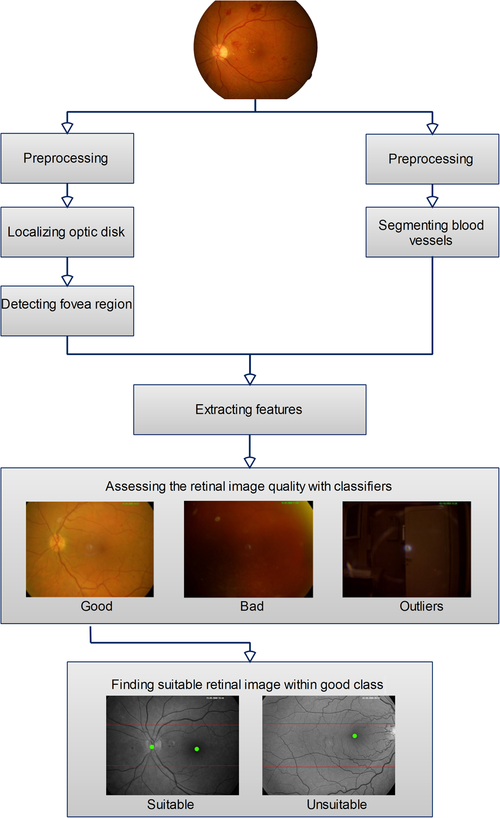
All the images used in DRIMDB are obtained from the Retina Department of Ophthalmology, Medical Faculty, Karadeniz Technical University. Furthermore, all images were obtained with a Canon CF-60UVi Fundus Camera using 60 deg FOV and stored in JPEG files at resolution. We designed our quality scale considering its simplicity and efficiency. In particular, we included an outlier class to identify the nonretinal images that could have been obtained for several reasons, such as wrong focus or patient absence. Then, we divided the images into two groups, which are good- and bad-quality images. It is important to note that retinal images with good quality in DRIMDB are medically suitable image candidates. We developed a two-step IQA approach to find MSRIs. The first step of our approach aims to identify the good retinal images, which are worthy of further analysis. The second step of our approach identifies medically suitable images among the goodquality retinal images. In the first step, we used DRIMDB to measure the classification performance of our approach. In addition, we used two additional public retinal image datasets [Digital Retinal Images for Vessel Extraction (DRIVE) and Standard Diabetic Retinopathy Database Calibration level 1 (DIARETDB1)8,9] in our experiments to identify MSRIs. Given that medical experts utilize these public datasets, we assume that each image is a medically suitable image for our experimental setups. The details of our approach are shown in Fig. 1 and are described in detail in the subsequent sections. Briefly, our approach consists of six phases. Initially, we enhanced an image’s visual information using image processing techniques to increase the visibility of crucial anatomical structures. This was followed by the feature extraction phase. Then, the image features were classified using machine learning methods to grade retinal images according to our quality scale. Finally, MSRIs were identified within the images classified as being of good quality. 2.1.PreprocessingThe visibility and clarity of blood vessels play an important role in assessing the retinal image quality. We applied image processing techniques to retinal images in order to enhance the visibility of blood vessels. Retinal images are generally stored in JPEG files using the RGB color space. According to many works in this area,10 the green channel of the retinal images contains the most valuable data because of its informative contrast rate. Hence, we extracted the green channel of the retinal image initially [Fig. 2(a)]. We inverted the gray level values of the green channel data to improve the visibility of blood vessels. Then, we stretched the contrast of the inverted green channel image. Given that the concavity of the posterior pole causes intensity variations in retinal images, we applied contrast-limited adaptive histogram equalization (CLAHE)11 to adjust the intensity distribution uniformity of the retinal image [Fig. 2(b)]. Fig. 2Blood vessel segmentation phases: (a) original green channel retinal image, (b) applying contrast-limited adaptive histogram equalization transform to inverse of green channel retinal image, (c) applying the morphological methods, (d) binarization of (c) with a triangle automatic threshold method, (e) removal of small region without vessels, and (f) overlaying the segmented vessels on the original green channel retinal image. 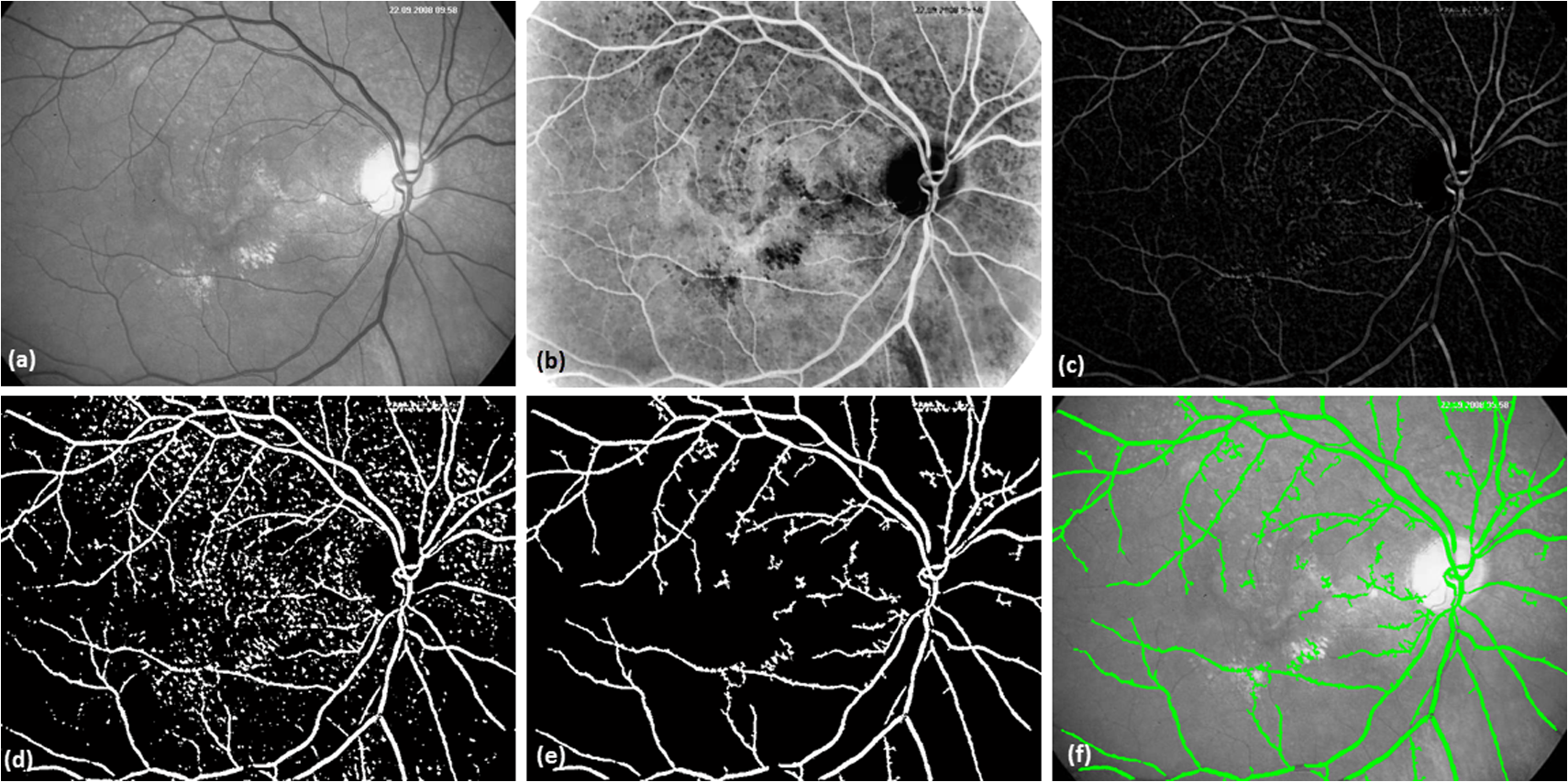 2.2.Segmentation of Retinal Blood VesselsThe preprocessing goal is to improve the visibility of blood vessels in the segmentation process. We preferred to use Zana and Klein’s vessel segmentation approach12 because of its simplicity and robustness. The method has a high accuracy and efficiency on the vessel segmentation process in retinal images. In detail, the method uses simple morphological operators to extract blood vessels of a retinal image. 2.3.OD DetectionOne of the most important steps of our approach is the OD detection step because it plays an important role in both retinal IQA and identification of MSRI processes.13,14 First, we used the visibility of the OD to identify the goodquality images because these images should contain the OD properly. Afterward, we determined that the location of the OD should be within a specific boundary in order to diagnose the retinal diseases on the posterior pole. The OD can be detected easily in a retinal image because of its unique features, such as high-intensity value and circularity. However, retinal images might contain such abnormalities that could be extremely similar to the OD. A simple threshold segmentation method might produce inaccurate results in this case. In our method, we used the vertical edge information to detect the OD because the OD is the vertical junction of vessels in a regular retinal image [Fig. 3(a)]. Therefore, it is expected that there should be several vertical edges around the OD. We used a vertical Sobel operator to extract the vertical edge information of preprocessed retinal images [Fig. 3(b)]. We calculated the vertical edge histogram using the following formula where VEH denotes vertical edge histogram, VI is the result of the vertical Sobel operator, denotes the total number of rows in VI, and and denote the row and column numbers of the image, respectively. The maximum value index of this histogram is an approximation of the horizontal center of the location of the OD. Therefore, we were able to reduce our OD search area from the entire retinal image to a neighborhood of two OD diameters of maximum value index. In other words, the horizontal center of the OD should remain within , where , , and [Fig. 3(b)].Fig. 3Detecting candidate area of the optic disk: (a) original image, (b) vertical edge histogram, and candidate optic disc (OD) region of the image.  Once the candidate region was determined, we extracted the candidate region image from the green channel image and adjusted the gray scale values of the target region [Figs. 4(a) and 4(b)]. We used the Canny edge detection operator to find edges in the target region [Fig. 4(c)]. Successively, we used the Hough transform to find circles in the edge image [Fig. 4(d)]. The Hough transform is an accumulation method defined as where is the center point of the circle being tested, is the radius of circle, and are the total number of rows and the total number of columns of the edge image, respectively, and is a binary function defined as where is the pixel value of the edge image at the point.15 We selected the maximum accumulator value of the Hough transform as the OD.16 The result of our OD detection approach is depicted in Fig. 4(e).2.4.Fovea DetectionThe fovea, which is the darkest part of a normal retinal image, is located at the center of the macula. In a formal manner, the location of the fovea remains within a ring between the two circles that have the same center as the OD and that have the radius of two and three OD diameters, respectively.17 Hence, we created a ring-shaped mask to locate the fovea that is depicted in Fig. 5(b). We used morphological closing to eliminate the side effects of retinal diseases and to increase the separability of the fovea. The best approximation of the fovea center is the location of the darkest point in the mask. Figure 5(c) shows the identified fovea and its neighborhood in the mask. Finally, we were able to locate the rest of the fovea components as shown in Fig. 5(d).18 2.5.Feature Extraction for Retinal IQAIn this work, we extracted a total of 177 features from a retinal image in order to determine the quality of an image. Our features can be categorized into three groups: shape, texture, and intensity. Shape features aim to represent the shape information of a segmented binary image. Given that we previously segmented a retinal image, we can use the shape features of the segmented image to express the vessel structure of the retina. We chose two shape features: one is called the inferior, superior, nasal, and temporal (ISNT) quadrant features19 and the other is the Zernike moments,20 which are expected to have high descriptive power. Moreover, the ISNT quadrant features and the Zernike moments describe the local and global properties of the vessel structure, respectively. Our goal is to identify the retinal images, as well as the nonretinal images obtained from fundus cameras. It is obvious that the texture of both types of images should be different from each other. Hence, we used texture features to distinguish retinal images from nonretinal images. Texture features model the repeating patterns of a local pixel intensity variation in an image. In this work, we used Haralick texture features, which aim to describe the texture globally,21 and the edge histogram, which expresses the texture locally.22 Finally, we used two color-related features to represent the color information of the images. The first feature is concerned with the pixel intensity distribution properties of a retinal image. It is expected that the histogram distribution of the high quality retinal image should be similar to a normal distribution. Therefore, we calculated the high-order statistical properties of the gray level histogram to represent the intensity distribution of a retinal image. The second feature represents the dominant color of the image in both the RGB and gray scale color spaces. 2.5.1.Regional features of ISNT quadrantsThe ISNT quadrants features represent the vessel structure of a retinal image in the four ISNT regions.19 The vessel information at each region is represented by shape descriptors. Hence, we extracted localized shape properties of vessel distribution in a retinal image with the help of these features. After segmenting the blood vessels, we created four masks to extract the ISNT regions. We calculated the area, major and minor axis lengths, eccentricity, orientation, Euler number, circle diameter, solidity, extent, and the perimeter properties of each region. In addition, high-quality retinal images should have a uniform vessel distribution among these quadrants. Consequently, we calculated two additional features from the ISNT quadrants, which are given in the following formulas: Figure 6 shows a graphical representation of the ISNT features. 2.5.2.Zernike momentsZernike polynomials20 are used to extract the global shape information of an image. They provide robust shape information that is invariant to rotation and scale. In mathematics, the Zernike moments are orthogonal moments that use the unit vector representation of an image. They are denoted as in the following formula: where denotes the absolute value of a real number, is the length of the vector from the origin to point , is the angle from the -axis to the vector, and . Here, are the Zernike polynomials and are denoted as in the following formula: whereWe used the first 15 Zernike polynomials to assess the global quality of retinal images in this work because they provide higher accuracy rates for shape-based classification tasks. 2.5.3.Gray level co-occurrence matrix featuresThe features of the gray level co-occurrence matrix (GLCM) were proposed by Haralick et al.21 It is intensively used in many texture-related studies. These features describe the texture using spatial intensity dependencies. In the original work, texture was defined by calculating the statistical properties of GLCM that represent intensity value co-occurrences at -distance and angle. As a result, GLCM is a square matrix whose rows and columns represent gray level intensity values. In other words, the size of the GLCM matrix depends on the number of gray levels in the image. The GLCM matrix is calculated using the following formula: where is the image function, and are the image width and height, and and are the distance parameters defined by and , respectively.After calculating the co-occurrence matrix, each element of the matrix is normalized using the following formula to create a normalized co-occurrence matrix [] where denotes the number of gray levels in the image and , which is also denoted as , is the ’th element of the normalized co-occurrence matrix.We used seven Haralick feature functions: contrast, correlation, sum of average, entropy, homogeneity, inverse difference moment, and maximum probability; they are computed at 0, 45, 90, and 135 deg angles for distance value one. 2.5.4.Edge histogram descriptorEdge information in an image can describe both shape and texture. We used the edge histogram descriptor, which is an element of the MPEG-7 standard, to extract the primitive information of the edge distribution.23,24 First, the retinal image was divided into 16 () subimages. A histogram of five standardized edge directions, shown in Fig. 7, was computed for each subimage. Fig. 7Filters used to determine edges (a) horizontal edge filter, (b) vertical edge filter, (c) 45-deg edge filter, (d) 135-deg edge filter, and (e) nondirectional edge filter. 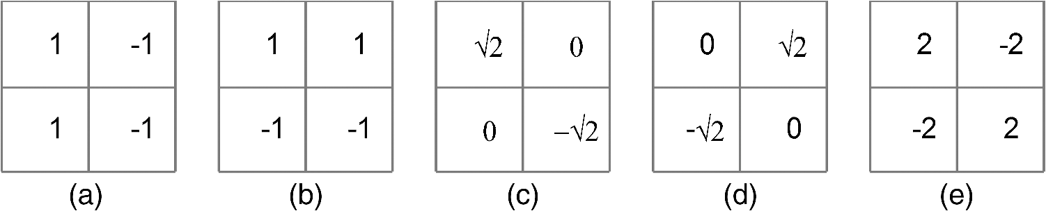 The edge histogram was calculated using the edge filter responses at each nonoverlapping blocks of each subimage. A block was assigned to the edge whenever the filter response was a maximum value. Hence, the number of elements in the edge histogram feature is 80 (the union of five bin histograms of each 16 subimage). 2.6.Finding a Suitable Retinal ImageIn this paper, we propose a method to determine MSRIs that include the OD, fovea, and superior and inferior arcades. MSRIs provide valuable information about the retina and are preferred by ophthalmologists. We call a retinal image an MSRI when it has both the OD and the fovea at a specific location called the expected region of OD (EROD). An example of EROD is depicted in Fig. 8. Fig. 8Examples of EROD (a) optimal boundaries for EROD (b) an example of retinal image having OD and fovea in EROD.  The EROD upper and lower bounds are calculated using the following formulas: where is vertical centerline of the retinal image, is the diameter of the OD, and and denote the lower and upper bounds of EROD, respectively. We called an image MSRI if it has both the OD and the fovea within EROD. Furthermore, we defined a new suitability metric for retinal images, which is calculated using the following formula: where is the component of the OD position. Hence, our metric decreases when the center of the OD approaches the image’s centerline.2.7.Performance Measurement of Retinal IQAWe implemented our feature extraction code using the MATLAB software. We executed the DRIMDB feature extraction on two different computer configurations (PC1 and PC2). PC1 has Intel Core i7 3770 quad-core CPU with 16 GB of RAM, and PC2 has Intel Core i7 3930K six-core CPU with 16 GB of RAM. We repeated feature extraction experiments 10 times to eliminate the cache effect using serial and parallel implementations. Moreover, we calculated the speed-up and efficiency scores for parallel implementation of the feature extraction process. The results of our experiments are listed in Table 2. Table 2Time analysis for feature extraction of images in DRIMDB.
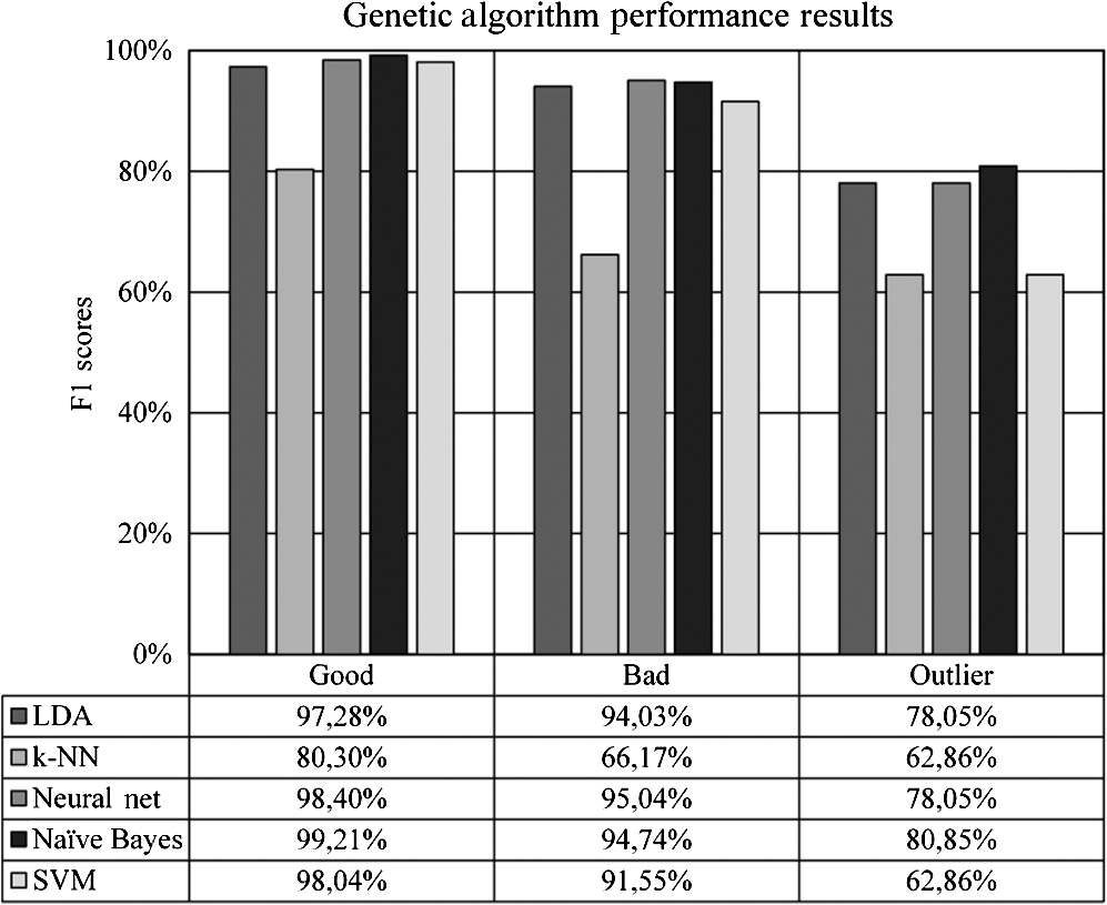
In this study, we measured the classification performance of the features described in Sec. 2.5 on the IQA task with the help of a data mining software.25 In addition, we conducted experiments to identify the best machine classifier for the retinal IQA task among five well-known machine classifiers: the linear discriminant analyze (LDA) with principal component analysis (PCA),26,27 the k-Nearest Neighbor28 (k-NN), the Neural Network (NN),29 the Naïve Bayes,30 and the support vector machines (SVMs).31 Some of these classifiers require parameters to be adjusted. We tested several parameter configurations to find the optimum parameter values. Furthermore, we used 10-fold cross-validation to ensure the objectivity of each experiment. We used PCA to manage the singularity problem of the LDA classifier. However, we had to adjust the PCA component count of the LDA+PCA classifier. Our experiments showed that the optimum parameter value of the PCA component count is 77. It is also noticeable that the best value for the k-NN classifier is found at one. We used one hidden layer for the NN classifier and calculated the hidden layer size using the input vector length and class count. We used Laplace correction to prevent the high influence of zero probabilities on Naïve Bayes experiments. The SVM classifier was the only binary classfier in our experiments. We used one-versus-all approach on experiments related with the SVM classifier, and our experiments show that the best value for the SVM classifier is . All our initial tests were performed on the combined vector of all the features explained in this paper. Classification performance can be degraded by feature vector dimension. This negative effect is known as the “curse of dimensionality.” There are two common methods to overcome this issue: selecting the most valuable features from the original subset and transforming the feature space into an effective low-dimensional one. These two methods are called feature selection and dimensionality reduction, respectively. Because we are considering a vector whose size is 177, we must ensure that our experiments are not affected by the curse of dimensionality side effect. We performed two feature selection approaches: a genetic algorithm32 and a forward selection33 method. All the experiments were executed on PC1. The time comparison of the methods is listed in Table 3. Table 3Time comparison of feature selection methods.
Most of the classification-related studies are concerned with assessing samples in two distinct classes called the binary classification systems. There are state-of-the-art evaluation metrics available in the literature to measure the performance of binary classification systems, such as receiver operating characteristics analysis, sensitivity, and specificity. However, our task requires evaluation metrics capable of measuring the performance of multiclass classifications. The most preferred metrics used for this task are precision and recall. Precision determines the rate of correctly predicted samples among classification results and recall determines the rate of correctly classified samples among actual samples (in some studies, recall is referred to as sensitivity).34 However, these two metrics can show different characteristics in some experiments. Therefore, we chose the F1 measure, which is the harmonic mean of precision and recall, to measure the performance of our experiments.34 As a result, we are able to identify the experimental setups obtaining high classification accuracy, as well as high predictive power. The formal definition of the F1 metrics is given in the following formula: 3.ResultsOur initial experimental results are presented in Fig. 9. According to the results, the SVM classifier slightly outperformed other classifiers at experiments on good and outlier classes with 99.60% and 84.21% F1 scores, respectively, whereas the LDA classifier outperformed other classifiers at experiments on the bad class with 97.78% F1 score. Although two different classifiers presented different characteristics on different classes, we suggest the use of the SVM classifier because of its overall classification success rate. Furthermore, we tested the performance effect of the dimensionality reduction approaches on the IQA task. Figures 10 and 11 depict the classification results of the genetic and forward feature selection approaches, respectively. According to the results, the feature selection methods increase the success rates of probabilistic classifiers. For example, the classification performance of the Naïve Bayes classifier increases with the help of the feature selection, as does the LDA classifier. It is also noticeable that the performance of the k-NN classifier increases considerably using the forward selection approach. However, the performance of some classifiers degraded for specific classes, according to our results. In particular, the classification performance of the experiments on the outlier class had the worst performance scores at feature selection tests of the SVM and NN classifiers. The main cause of this issue is closely related to the number of samples that belong to the outlier class because it has the smallest sample size compared to the other quality classes. Reducing the dimension might remove information, which is crucial for outlier detection. In addition, the feature selection approach increased the overall performance rates of the LDA classifier noticeably among other classifiers. The classification performance of the LDA classifier measured at 98.81%, 96.40%, and 85.00% for the good, bad, and outlier classes, respectively. Although individual classification performances of classifiers varied with the quality classes, the SVM classifier obtained the optimum classification performance scores without any feature selection method considering the overall classification performances. Moreover, we performed additional tests to determine whether the image fits our MSRI condition. Hence, after assessing the quality of an image, we performed further experiments to measure the performance of our MSRI detection approach on DRIMDB, DRIVE, and DIARETDB1 and obtained 97.60%, 100.0%, and 96.63% of detection rates, respectively. The performance scores of our approach are listed in Table 4. Table 4Performance scores of MSRI detection approach.
Figure 12 shows the successful and failed sample images for DRIMDB and DIARETDB1, respectively. Each image includes red dots that represent our OD and fovea detection results. Moreover, the EROD boundaries are presented in each image with red lines. Given that our approach depends on an accurate OD position, any image transformation related to the OD position will have a negative impact on our results. For example, the image frame of the DRIMDB failed sample includes an incomplete OD. Hence, our approach found the OD location incorrectly. In addition, our approach was unable to find fovea. Furthermore, the DIARETDB1 failed sample has extremely unbalanced spatial intensity distribution. So, our approach only found the location of the OD correctly. Besides, our approach could successfully find the exact location of the OD and fovea on the images given in Figs. 12(a) and 12(c). Fig. 12Successful and failed samples from DRIMDB and DIARETDB1 (a) DRIMDB successful sample, (b) DRIMDB failed sample, (c) DIARETDB1 successful sample, and (d) DIARETDB1 failed sample.  Our approach requires good-quality retinal images to detect the fovea. We inspected each image in the DRIMDB for their qualities. However, we used each image in the DIARETDB1 directly in our MSRI detection approach. Because the DIARETDB1 has no quality information, our approach fails to detect the exact location of the fovea in images in the DIARETDB1 where there is an insufficient contrast rate. 4.DiscussionThe most important anatomical structures of the retina are the vessels, OD, macula, and vascular arches. MSRIs should contain all the important retinal structures as much as possible and should ensure that those structures are as clear as possible. Successful retinal diagnosis depends on the clarity of the retinal structures. However, the clarity of the retinal image is insufficient without a proper image frame. In this paper, we presented a novel approach to identifying the retinal images with a good clarity and a proper frame. Hence, automatic retinal image analysis systems can acquire high accuracy rates using these images. In fact, several retinal images acquired in clinical systems have insufficient information to diagnose the retinal diseases. These images are useless for automated image analysis systems and occupy redundant disc space. This issue can be resolved by assessing the image quality with the help of automated IQA approaches, before such images are saved into automatic retinal image analysis systems. Therefore, the valuable time of ophthalmologists can be saved by eliminating the inadequate retinal images. In other words, IQA will improve both the quality and the time efficiency of the retinal image diagnostic process. Most of the current studies measure the retinal image quality with the help of vessel densities or intensity variations.2–7 Additionally, some studies discard nonretinal image identification and are concerned only with retinal image quality. However, nonretinal images can have a negative impact on automatic retinal analysis systems and increase the rate of false positives. For instance, Fleming et al.3 and Paulus et al.2 discarded outlier images and categorized retinal image quality. Paulus et al.2 used Haralick et al.21 texture features and reported 92.7% of an area under curve (AUC) rate. Wen et al.35 proposed an IQA approach using blood vessel information. However, they ignored the contrast and color saturation knowledge of retinal images. Fleming et al.3 proposed a complex metric table for IQA. Although they presented more quality classes than we do in this paper, Fleming et al.3 propose one bad class and more than one good classes. In other words, there is no outlier class that contains nonretinal images in their grading system. On the other hand, some works attempt to detect nonretinal images. For instance, Giancardo et al.4 include the outlier images in their study, but the success rate of their outlier detection is 80%, caused by detecting false vessel-like structures in the outlier images. Moreover, some retinal images were labeled as outlier because of their insufficient diagnostic data. Lalonde et al.5 propose an outlier detection system based on local pixel intensity distribution. The approach is open to errors for images that possess similar intensity distributions. In our paper, we proposed a two-phased MSRI detection approach. First, we graded the quality of retinal images; then, we identified MSRI images among good-quality images. Our approach provides a better identification scheme for images that can be used in the retinal diagnostic process. There are several reports on the success rates of visual features for different medical imaging systems in the literature.36 However, our current works on retinal imaging generally involve new features instead of existing ones.3,4,18 Specific visual features for problems are thought to be more efficient, although the existing features have high success rates for different applications.37–39 Moreover, the existing features can be integrated easily into any visual analysis system. Hence, the performance evaluation of the existing visual features will provide more valuable information for the literature. Another aspect of our work is to find the most suitable visual features for the retinal IQA task. In addition, we proposed two novel simple and robust features for measuring the accuracy of the image frame. We selected our visual feature to represent both local and global properties of the retinal images in terms of texture and shape. In other words, we analyzed the shape and texture information of retinal images at the local and global scales. Finally, we presented our experimental results, and our feature-set obtained extremely high accuracy rates. In this work, we proposed a new MSRI metric, which is exceedingly simple and robust. According to the experimental results, our MSRI metric obtained at least a 96% true detection rate. Hence, our approach identifies the MSRI images with high sensitivity scores. Our approach can be integrated into any retinal image diagnostic system easily. Furthermore, our approach can increase both the efficiency and accuracy of the retinal image diagnostic process. In conclusion, we can say that the robustness of automatic retinal image analysis systems can increase with the help of our approach. AcknowledgmentsThe authors would like to thank the Ophthalmology Department of Karadeniz Technical University, the Image Sciences Institute of the University Medical Center Utrecht, and the Machine Vision and Pattern Recognition Laboratory of the Lappeenranta University of Technology for allowing us to use their retinal image databases. ReferencesC. Köseet al.,
“Simple methods for segmentation and measurement of diabetic retinopathy lesions in retinal fundus images,”
Comput. Methods Programs Biomed., 107
(2), 274
–293
(2012). http://dx.doi.org/10.1016/j.cmpb.2011.06.007 CMPBEK 0169-2607 Google Scholar
J. Pauluset al.,
“Automated quality assessment of retinal fundus photos,”
Int. J. Comput. Assist. Radiol. Surg., 5
(6), 557
–564
(2010). http://dx.doi.org/10.1007/s11548-010-0479-7 1861-6410 Google Scholar
A. D. Fleminget al.,
“Automated assessment of diabetic retinal image quality based on clarity and field definition,”
Invest. Ophthalmol. Vis. Sci., 47
(3), 1120
–1125
(2006). http://dx.doi.org/10.1167/iovs.05-1155 IOVSDA 0146-0404 Google Scholar
L. Giancardoet al.,
“Elliptical local vessel density: a fast and robust quality metric for retinal images,”
in Conf. Proc. IEEE Eng. Med. Biol. Soc.,
3534
–3537
(2008). Google Scholar
M. LalondeL. GagnonM. Boucher,
“Automatic visual quality assessment in optical fundus images,”
in Proc. of Vision Interface,
259
–264
(2001). Google Scholar
S. C. LeeY. Wang,
“Automatic retinal image quality assessment and enhancement,”
Proc. SPIE, 3661 1581
–1590
(1999). http://dx.doi.org/10.1117/12.348562 Google Scholar
M. NiemeijerM. D. AbràmoffB. van Ginneken,
“Image structure clustering for image quality verification of color retina images in diabetic retinopathy screening,”
Med. Image Anal., 10
(6), 888
–898
(2006). http://dx.doi.org/10.1016/j.media.2006.09.006 MIAECY 1361-8415 Google Scholar
J. Staalet al.,
“Ridge-based vessel segmentation in color images of the retina,”
IEEE Trans. Med. Imaging, 23
(4), 501
–509
(2004). http://dx.doi.org/10.1109/TMI.2004.825627 ITMID4 0278-0062 Google Scholar
T. Kauppi,
“Eye fundus image analysis for automatic detection of diabetic retinopathy,”
(2010). Google Scholar
Y. WangW. TanS. C. Lee,
“Illumination normalization of retinal images using sampling and interpolation,”
Proc. SPIE, 4322 500
–507
(2001). http://dx.doi.org/10.1117/12.431123 Google Scholar
A. M. Reza,
“Realization of the contrast limited adaptive histogram equalization (CLAHE) for real-time image enhancement,”
J. VLSI Signal Process. Signal, Image Video Technol., 38
(1), 35
–44
(2004). http://dx.doi.org/10.1023/B:VLSI.0000028532.53893.82 1387-5485 Google Scholar
F. ZanaJ. C. Klein,
“Segmentation of vessel-like patterns using mathematical morphology and curvature evaluation,”
IEEE Trans. Image Process., 10
(7), 1010
–1019
(2001). http://dx.doi.org/10.1109/83.931095 IIPRE4 1057-7149 Google Scholar
S. SekharW. Al-NuaimyA. K. Nandi,
“Automated localisation of retinal optic disk using Hough transform,”
in 2008 5th IEEE Int. Symp. Biomed. Imaging From Nano to Macro,
1577
–1580
(2008). Google Scholar
M. U. Akramet al.,
“Retinal images: optic disk localization,”
in Int. Conf. Image Anal. Recognit.,
40
–49
(2010). Google Scholar
S. LiangwongsanB. Marungsri,
“Extracted circle hough transform and circle defect detection algorithm,”
World Acad. Sci. Eng. Technol., 5
(12), 316
–321
(2011). Google Scholar
C. KöseU. SevikO. Gençalioğlu,
“Automatic segmentation of age-related macular degeneration in retinal fundus images,”
Comput. Biol. Med., 38
(5), 611
–619
(2008). http://dx.doi.org/10.1016/j.compbiomed.2008.02.008 CBMDAW 0010-4825 Google Scholar
C. Sinthanayothinet al.,
“Automated localisation of the optic disc, fovea, and retinal blood vessels from digital colour fundus images,”
Br. J. Ophthalmol., 83
(8), 902
–910
(1999). http://dx.doi.org/10.1136/bjo.83.8.902 BJOPAL 0007-1161 Google Scholar
J. NayakP. S. BhatU. R. Acharya,
“Automatic identification of diabetic maculopathy stages using fundus images,”
J. Med. Eng. Technol., 33
(2), 119
–129
(2009). http://dx.doi.org/10.1080/03091900701349602 JMTEDN 0309-1902 Google Scholar
J. Nayaket al.,
“Automated diagnosis of glaucoma using digital fundus images,”
J. Med. Syst., 33
(5), 337
–346
(2009). http://dx.doi.org/10.1007/s10916-008-9195-z JMSYDA 0148-5598 Google Scholar
S.-K. HwangW.-Y. Kim,
“A novel approach to the fast computation of Zernike moments,”
Pattern Recognit., 39
(11), 2065
–2076
(2006). http://dx.doi.org/10.1016/j.patcog.2006.03.004 PTNRA8 0031-3203 Google Scholar
R. M. HaralickK. ShanmugamI. H. Dinstein,
“Textural features for image classification,”
IEEE Trans. Syst. Man Cybern., 3
(6), 610
–621
(1973). http://dx.doi.org/10.1109/TSMC.1973.4309314 ISYMAW 0018-9472 Google Scholar
B. S. Manjunathet al.,
“Color and texture descriptors,”
IEEE Trans. Circuits Syst. Video Technol., 11
(6), 703
–715
(2001). http://dx.doi.org/10.1109/76.927424 ITCTEM 1051-8215 Google Scholar
D. K. ParkY. S. JeonC. S. Won,
“Efficient use of local edge histogram descriptor,”
in Proc. 2000 ACM Work. Multimed.,
51
–54
(2000). Google Scholar
C. S. Won,
“Feature extraction and evaluation using edge histogram descriptor in MPEG-7,”
583
–590
(2004). Google Scholar
I. Mierswaet al.,
“YALE: rapid prototyping for complex data mining tasks,”
in Proc. 12th ACM SIGKDD Int. Conf. on Knowledge Discovery and Data Mining,
935
–940
(2006). Google Scholar
S. Mikaet al.,
“Fisher discriminant analysis with kernels,”
in Proc. 1999 IEEE Signal Process. Soc. Work.,
41
–48
(1999). Google Scholar
J. YangJ. Yang,
“Why can LDA be performed in PCA transformed space?,”
Pattern Recognit., 36
(2), 563
–566
(2003). http://dx.doi.org/10.1016/S0031-3203(02)00048-1 PTNRA8 0031-3203 Google Scholar
D. Bremneret al.,
“Output-sensitive algorithms for computing nearest-neighbour decision boundaries,”
Discrete Comput. Geom., 33
(4), 593
–604
(2005). http://dx.doi.org/10.1007/s00454-004-1152-0 0179-5376 Google Scholar
H.K.D.H. Bhadeshia,
“Neural networks in materials science,”
ISIJ Int., 39
(10), 966
–979
(1999). http://dx.doi.org/10.2355/isijinternational.39.966 IINTEY 0915-1559 Google Scholar
H. Zhang,
“The optimality of Naive Bayes,”
in Proc. 17th Int. FLAIRS Conf.,
562
–567
(2004). Google Scholar
C. CortesV. Vapnik,
“Support-vector networks,”
Mach. Learn., 20
(3), 273
–297
(1995). http://dx.doi.org/10.1007/BF00994018 MALEEZ 0885-6125 Google Scholar
W. SiedleckiJ. Sklansky,
“A note on genetic algorithms for large-scale feature selection,”
Pattern Recognit. Lett., 10
(5), 335
–347
(1989). http://dx.doi.org/10.1016/0167-8655(89)90037-8 PRLEDG 0167-8655 Google Scholar
P. PudilJ. NovovičováJ. Kittler,
“Floating search methods in feature selection,”
Pattern Recognit. Lett., 15
(11), 1119
–1125
(1994). http://dx.doi.org/10.1016/0167-8655(94)90127-9 PRLEDG 0167-8655 Google Scholar
D.M.W. Powers,
“Evaluation: from precision, recall and f-measure to roc., informedness, markedness & correlation,”
J. Mach. Learn. Technol., 2
(1), 37
–63
(2011). 2229-3981 Google Scholar
Y.-H. WenA. Bainbridge-SmithA. B. Morris,
“Automated assessment of diabetic retinal image quality based on blood vessel detection,”
in Proc. Image Vis. Comput.,
132
–136
(2007). Google Scholar
H. Mülleret al.,
“A review of content-based image retrieval systems in medical applications-clinical benefits and future directions,”
Int. J. Med. Inform., 73
(1), 1
–23
(2004). http://dx.doi.org/10.1016/j.ijmedinf.2003.11.024 1386-5056 Google Scholar
N. A. Rosaet al.,
“Using relevance feedback to reduce the semantic gap in content-based image retrieval of mammographic masses,”
in Proc. 30th Annu. Int. Conf. IEEE Eng. Med. Biol. Soc.,
406
–409
(2008). Google Scholar
B. Zheng,
“Computer-aided diagnosis in mammography using content-based image retrieval approaches: current status and future perspectives,”
Algorithms, 2
(2), 828
–849
(2009). http://dx.doi.org/10.3390/a2020828 ALGOCH 1999-4893 Google Scholar
D. D. Feng,
“Automatic medical image categorization and annotation using LBP and MPEG-7 edge histograms,”
in 2008 Int. Conf. Technology & Biomedical Application,
51
–53
(2008). Google Scholar
BiographyUğur Şevik received a BS degree in statistics and computer science in 2003, a MS degree in 2007, and is a PhD candidate in computer engineering at the Karadeniz Technical University, Trabzon, Turkey. He has been a research assistant at the Department of Statistics and Computer Science, Karadeniz Technical University, Trabzon, Turkey, since 2005. His research interests include image processing, pattern recognition, statistical learning, data mining, retinal image analysis, and forestry management systems. Cemal Köse received his BS and MS degrees in the Department of Electrical and Electronic Engineering from Karadeniz Technical University, Trabzon, Turkey, in 1986 and 1990, respectively. He received a PhD in the Department of Computer Science from the University of Bristol, Bristol, UK, in 1997. He is currently an associate professor in the Department of Computer Engineering, Karadeniz Technical University, Trabzon, Turkey. His research interests include parallel processing, pattern recognition, natural language processing, and computer graphics. Tolga Berber received his BS degree in statistics and computer science from Karadeniz Technical University in 2002 and a PhD degree in computer engineering from Dokuz Eylul University in 2013. He has been working at the Department of Statistics and Computer Science, Karadeniz Technical University, since 2013. His current research interests include information retrieval, machine learning, image analysis, text mining, pattern recognition, and multimedia databases. Hidayet Erdöl graduated from Istanbul University, Faculty of Medicine, Turkey, in 1988. He was a resident physician in the Department of Ophthalmology, Karadeniz Technical University from 1990 to 1995. He has been a professor of medicine in the same department since 2010. He has been the head of the Ophthalmology Department since 2007. His research interests include glaucoma, diabetic retinopathy, age-related macular degeneration, and retinal diseases. |
|||||||||||||||||||||||||||||||||||||||||||||||||||||||||||||||||||||||||||||||||