2.1.

Experimental Setup

The study of the CSD events in rats’ cortex involved the preparation of the experimental setup and the animal for the measurements. The experimental setup for concurrent use of BPI, OIS imaging, and electrophysiological recordings comprises of two principal parts: recording systems (optical and electrophysiological) and the animal unit (stereotaxis, heating control, etc.) with rat. The schematic drawing of the whole experimental setup is shown in Fig. 1(a). The optical system for implementation of both the BPI and OIS techniques includes two optical elements: a photodetector and an illuminator. As the photodetector, we used a digital, monochrome 8-bit CMOS camera (EO-1312, Edmund Optics, Barrington, New Jersey) with attached camera lens (18 to 108 mm focal length, Canon, Tokyo, Japan). Video frames with size of $300\times 300\text{pixels}$ were recorded at the rate of $60\text{frames}/\mathrm{s}$.

Fig. 1

(a) Layout of the experimental setup with blood pulsation imaging of the rat cortex: P1, P2—polarizers, E1, E2—local field potential (LFP) electrodes, implanted into the right and left hemispheres, LED—light emitted diode ($\lambda =920\mathrm{nm}$). (b) Schematic view of the rat head with overlaid raw camera image showing the KCl-application site and the location of the LFP electrodes E1, E2.

As illuminator, we used a conventional light-emitting diode (LED) (H2A1-H920, Roithner Lasertechnik GmbH, Wien, Austria) that generated the light at the wavelength of 920 nm. This wavelength was chosen because we found that the SNR for rat cortex illumination is higher compared with illumination by LEDs operating at the wavelength from the visible range. Moreover, the penetration depth in the tissue of the infrared light is larger than that of the visible light.²⁸ The optical power of the LED is 80 mW, the wavelength bandwidth is 60 nm. The illuminator provided uniform illumination of the open skull area sizing $3\times 3\mathrm{c}{\mathrm{m}}^2$ at a distance between the subject and video camera of about 8 cm. Note that during video recording the lens diaphragm and the camera exposure time were adjusted so that the recorded frames did not contain saturated pixels (the maximal pixel value is 255 for 8-bit camera), but were as bright as possible. During the experiment, the ambient illumination was much lower than that provided by the illuminator.

The camera was mounted in a vertical position for recording the focused image of the rat’s cortex, and it was fixed so that the angle between the optical axis of the camera and illuminator was minimal. The generated light was linearly polarized by means of a polarizer P1 [Fig. 1(a)] attached to the illuminator. The polarizer P2 was attached to the camera lens so that its transmission axis was oriented orthogonal to the polarization vector of the illuminating light. By using crossed polarizations, we reject the light reflected from the cortex surface-air interface. The camera was connected to a personal computer (PC) through the universal serial bus (USB) port providing the frames transfer for downloading to the computer hard drive. The illuminator also was connected to the PC through other USB port for powering of the LEDs, which benefits in the full portability of the video recording system.

The electrophysiological recording was done by conventional LFPs technique using a BrainAmp MR Plus system (Brain Products GmbH, Munich, Germany). Signal from the electrodes E1 and E2 [Fig. 1(b)] was amplified, notch-filtered at 50 Hz and digitized with sampling rate of 5000 Hz. LFP recording system was connected to the same PC for real-time processing, monitoring, and storage of the data.

2.2.

Animal Preparation

Male Wistar rats 12 to 14 weeks old ($n=6$, National Laboratory Animal Center of the University of Eastern Finland) were used in this study. During surgical preparation procedures all rats were anesthetized with isoflurane (4% for induction and 2% for maintenance during surgery) in 70% ${\mathrm{N}}_2$—30% ${\mathrm{O}}_2$ mixture. Xylocaine gel was used to alleviate pain in incision and pressure points. Body temperature was maintained at approximately 37°C with a heating pad. Anesthetized rat was mounted into a stereotactic frame (David Kopf Instruments GmbH, Düsseldorf, Germany) for craniectomy and guided electrode implantation. The frame also served to avoid motion artifacts during the recording session after the surgery.

For optical imaging, the scalp was excised and skull bones were cleaned from soft tissues remainders with hydrogen peroxide solution (Sigma Aldrich GmbH, Munich, Germany). Parietal bones were bilaterally removed from sigma to bregma using a dental drill. The central strip of the skull along the suture was left untouched to avoid damaging of the sagittal sinus. Maximum care was taken to preserve integrity of meninges and prevent bleeding. After the surgery, isoflurane anesthesia was switched to urethane ($1.25\mathrm{g}/\mathrm{kg}$, Sigma Aldrich GmbH, Germany).

For LFP recordings two insulated tungsten 50-μm diameter electrodes (California Fine Wire, Grover Beach, California) were implanted into the left and right anterior cortex ($+1\text{-}\mathrm{mm}$ anterior from bregma, 2.5 mm from midline, at the depth of 0.5 mm from the surface of the brain). Permabond gel glue (Permabond Engineering Adhesives Ltd., Hampshire, United Kingdom) was used to fix the electrodes to the skull. Chloridized silver wire reference and ground electrodes were placed subcutaneously in the neck. Heart rate of the animals was preliminary assessed by a pulse oximeter (SA Instruments Inc., Stony Brook, New York). The heartbeat rate of animals was in the range of 360 to 480 beats per minute.

CSD was induced by topical application of 10 μl of 1-M KCl solution (Sigma Aldrich GmbH, Germany) onto occipital cortex area ($-6\mathrm{mm}$ from bregma, 3 mm lateral from midline). The total number of the KCl applications in six animals was 10. In two rats, we applied KCl only in the right hemisphere and in four rats the potassium chloride was applied first in the right hemisphere, then in the left one. One application evoked 1 to 4 CSD waves per experiment. Note that each KCl application was done as a separate statistically independent experiment because it was at least 25-min delay between KCl applications in different hemispheres of the same animal.

All animal procedures were approved by the National Ethical Committee for the Welfare of Laboratory Animals and conducted in accordance with the guidelines set by the European Community Council Directives 86/609/EEC. All means were taken to minimize the number of animals used and their suffering. Rats were group housed with preserved 12-h light/12-h dark cycle and ad libitum access to food and water. After the end of experiment, animals were sacrificed by intravenous injection of saturated K+ solution covered with 5% Isoflurane anesthesia.

2.3.

Procedure Protocol

Between the end of the surgery and beginning of the measurements all animals were kept in rest during 20 to 30 min to minimize the influence of postsurgical reaction on the obtained results. The duration of one measurement for each animal was 20 min. After initiation of the computer program, the camera began a continuous video recording of the focused area of the cortex. LFP recording was simultaneously started with the camera. After 1 min from the beginning of video recording, a drop ($\sim 10\mu \text{l}$) of KCl solution was applied manually using 0.1-ml syringe. Position of the LFP electrodes with respect to the location of KCl application, which is viewed in the video frame of the skull and exposed cortical surface overlaid with the rat’s head drawing, is shown in Fig. 1(b).

No manipulation with the animal and setup was done during next 19 min after KCl application while the illuminated cortex was continuously recorded by the camera. Note that both video stream and LFP recording were not interrupted during the KCl application. All the video frames and LFP data were stored in the PC for further processing.

2.4.

Blood Pulsation Imaging

The recorded video frames were processed by using custom software implemented in the MATLAB® platform. 2-D mapping of both the blood pulsation amplitude (BPA) and the relative phase of pulsations (BPP) was calculated using lock-in amplification of every pixel of the recorded video frames synchronously with a cardiac cycle.²⁴ The algorithm consists of two steps: (i) formation of the reference function and (ii) calculation of the correlation matrix representing 2-D distribution of BPA and BPP. The reference function was defined from the recorded frames as follows. We average pixels over the whole area of the open cranial window, which results in the PPG waveform from the whole series of the frames. As known,²⁹ the PPG waveform is temporally modulated at the heartbeat frequency, which allows us to define the duration, $T_C$, and beginning of each heartbeat. The reference function, $R(t)$, was defined for every cardiac cycle with its specific $T_C$ as

The coefficient $A_M$ was defined from the condition of the normalization

Thereafter, we calculated the correlation between temporal variations of each pixel in the series of recorded frames and the above defined reference function, $R(t)$, in the form of a correlation matrix $S_C(x,y)$:

Here, $I(x,y,t)$ is a value of the pixel with coordinates $(x,y)$ of the image frame captured at the moment of $t$. Both $R(t)$ and recorded frames used in Eq. (3) are associated with time moments from the interval of each cardiac cycle with duration $T_C$. The correlation matrix $S_C(x,y)$ contains the same number of pixels as any of the recorded frames $I(x,y,t)$. The modulus of each pixel value of the $S_C(x,y)$ matrix is proportional to the modulation amplitude of the light reflected back from the respective point at the cortex.²⁴ Since this modulation is caused by the blood pulsations related to the heart activity,³⁰ the modulus of the correlation matrix, $|S_C(x,y)|$, describes the spatial distribution of BPA after normalization with a value from the corresponding location of a time-averaged image matrix. Respectively, the argument of a complex value of the matrix $S_C(x,y)$ describes the spatial 2-D distribution of BPP.

2.5.

OISs Imaging

The same recorded frames were also used for calculation of OIS images, which represent 2-D spatial changes of CBV.^11,16 For visualization of the CSD wave, we calculated the difference image $D(x,y)$ (which is a rate-of-change image) using on the following equation:¹⁶

Here, $I_0(x,y)$ denotes the initial image just prior to the CSD wave, $I_i(x,y)$ refers to the image at the $i$’th time point, and $I_{i-1}(x,y)$ refers to the immediately previous image at the time point $i-1$. Each $I_i(x,y)$ image was obtained after averaging of the recorded frames within $\mathrm{\Delta }t$ interval to increase the SNR. The time step $\mathrm{\Delta }t$ between adjacent time moments was set to be equal to 40 cardiac cycles of the animal. Therefore, it was dependent on the heartbeat rate and varied in the range of 4 to 6.5 s. The difference imaging was shown to significantly enhance the leading and trailing edges of the CSD wave.¹⁶

3.1.

Spatio-Temporal Dynamics of Blood Pulsations and OIS Images

From the recorded video frames, we calculated two arrays of the images. First was the series of the correlation matrices $S_C(x,y)$ obtained using Eq. (3), and the second was the series of difference images $D(x,y)$ obtained using Eq. (4). To increase SNR of BPA maps, we averaged the modulus of the correlation matrices (which were calculated for every cardiac cycle of an animal) within $\mathrm{\Delta }t$ equal to 40 cardiac cycles. The same $\mathrm{\Delta }t$ was used for calculating the OIS images. Therefore, the total number of averaged images was the same in both arrays. Any pair of the images was obtained by different techniques (BPI and OIS imaging) exactly at the same moment of time representing the spatio-temporal dynamics of both blood pulsations and CBV. Typical sequence of BPA maps and OIS images is shown in Fig. 2 in the rows (a) and (b), respectively.

Fig. 2

Comparison of blood pulsations imaging (BPI) and optical intrinsic signal (OIS) images during cortical spreading depression (CSD) wave propagation through the brain cortex of rat #3 from the KCl application site which is marked by the red square: (a) blood pulsation amplitude (BPA) maps; (b) difference OIS images calculated for the same time moments; (c) constrictive; and (d) dilative CBV components of OIS images. Numbers above the columns indicate the time in seconds from the moment of KCl application. The actual size of presented BPA maps and OIS images is $15\times 15\mathrm{m}{\mathrm{m}}^2$.

As one can see from the row (b) of Fig. 2, OIS imaging technique reveals the CSD event as a wave originating from the site of topical application of KCl and radially propagating toward the periphery of the cortex. Such a wave was observed and reported by different research groups.^5,11–14,19 It typically consists of the bright region of increased reflectance due to decrease of CBV, which is followed by the darker hyperperfusion region of decreased reflectance caused by higher absorption of increased CBV. Figure 2(b) shows OIS images recalculated into the change of CBV so that the areas with increased CBV (dilated blood vessels) are colored by the red while those with reduced CBV (constricted vessels) are colored by the blue. For better visualization and analysis we show separately propagation of constriction and dilation waves in rows (c) and (d), respectively.

As seen in Fig. 2(a), an increase of the amplitudes in BPA maps appears after KCl application with the delay of about 90 s, which is approximately the same as for the dilation wave [Fig. 2(d)]. However, simultaneous appearance of BPA and dilative CBV was not observed in all animals. For quantitative estimation of the delay between the different vascular components, we used moments in which these components [being averaged in the regions of interest (ROI) centered with the area of KCl application] reach their extremes. Figure 3 shows the delay between vascular components in different animals. Symbols in the $x$-axis encrypt the rat’s number and the hemisphere in which KCl was injected: R—the right, and L—the left. Blue squares in Fig. 3(a) are the time when the constrictive wave of the primary CSD event reaches its minimum after KCl application in different rats. As seen, the latent period of the constrictive CBV component varies from 21 to 76 s. However, the delay time between the constrictive and dilative CBV waves is about the same ($47\pm 10\mathrm{s}$) for all rats as follows from the curve (b), red circles in Fig. 3. In contrast, the delay between the BPA component and dilative CBV component varies not only among different rats but also between different hemispheres of the same rat [see black triangles in Fig. 3(c)]. Note that in rat #1 the BPA wave is in the maximum very late when the dilative CBV wave was completely gone (the delay time is 42 s versus 18.5 s of the half width at the half height of the dilative CBV peak), but sometimes the BPA wave reaches its peak earlier than the dilative wave its dip (negative delay time in Fig. 3).

Fig. 3

Delay time of vascular components in different animals: (a) time required for the constrictive CBV component of primary CSD events to reach its dip after KCl application (blue squares); (b) delay time between the peak of the dilative and dip of the constrictive CBV components (red circles); (c) delay time between peaks of BPA and dilative CBV components (black triangles).

The BPA maps during their latent period do not differ from the maps calculated during the baseline (before KCl application). Although we did not observe high amplitude in the BPA maps during the baseline, the contours of both cranial windows are distinguishable in the background of all BPA maps compare to near-zero pulsation amplitudes of the skull. This allows us to estimate the SNR of BPA maps during the baseline being in the range of 2 to 3.

It is worth noticing that the increase of BPA does not cover the whole tissue of the cerebral hemisphere, in which the CSD was induced but occurs in the specific limited area in the temporal cortex. Therefore, we concurrently observed two different vascular components of the CSD event: (i) a CBV component visualized by OIS imaging and (ii) a BPA component revealed by BPI. The latter component migrates through the cortical tissue along an unusual trajectory (not radially).

We also evaluated the relative blood pulsation phase maps from the same correlation matrices as the BPA maps by accounting the argument of the matrix values. The variation of the BPP in the relative phase mapping associated with the time interval of the CSD wave was typically $13\pm 3\mathrm{deg}$. The variability of the BPP associated with a baseline time interval was at the level of $6\pm 2\mathrm{deg}$. This means that the use of the BPP mapping allows observation of the CSD event in parallel with BPA mapping. However, the increase of the BPP values in their maxima during CSD event with respect to variations of BPP during the baseline (before any KCl application) was $<2$. This is 5 to 8 times smaller than that of the BPA values. Therefore, the following results of the BPI technique are based on the BPA maps only.

3.2.

BPA Component of CSD Wave

As shown in Fig. 2(a), the BPA component of the CSD wave propagates mainly through the lateral area of a hemisphere (in the temporal cortex). Moreover, it originates from the place distant from the KCl-application site, which is in contrast with the CBV component originating from the application site. The BPA component is delayed with respect to the CBV component by a delay of about 90 s from the external impact [the image at 92 s in Fig. 2(a)], then it migrates along the cortex towards the animal’s nose with the amplitude diminishing after 169 s, and is recovered to the initial amplitude level (during the baseline) after 200 s. In two additional experiments, the CSD was induced in the rostral site close to the animal nose. In these cases, the BPA component propagated again along the similar trajectory in the lateral area of the hemisphere, as during caudal KCl application. However, the CSD propagation was in the opposite direction, toward the animal tail. CBV component in all cases propagated in the form of concentric rings outward the application site.

The trajectory of the BPA component of the CSD wave propagation can be estimated by calculating the coordinates of the “center of mass” of the migrating BPA area in Fig. 2(a). We found that the trajectory line connected the obtained points of the “center of mass” is of bow-shaped form. Such a nonlinear trajectory of the BPA component propagation was observed in all the experiments.

The trajectory of the BPA component can be also visualized by averaging of all correlation matrices during the CSD event [94 to 197 s in Fig. 2(a)]. The temporal averaging of these matrices results in single correlation matrix. The modulus of this matrix describes the spatial distribution of the mean BPA during propagation of the CSD wave. The BPA maps calculated for two different rats are shown in Figs. 4(a) and 4(b). In the same averaged BPA map, we placed the trajectory (black dotted line) obtained by evaluating the coordinates of the “center of mass” as it was described above. These maps show the spatial distribution of the BPA component during its propagation as increased amplitudes zones along the black dotted lines. The direction of the BPA component propagation was outwards the area of the KCl application and toward the anterior cortex of the rat as shown by arrows in Fig. 4. It is worth noting that the BPA component of the CSD wave appears in the same hemisphere, where the KCl was applied: in the right hemisphere in Fig. 4(a) and in the left one in Fig. 4(b).

Fig. 4

BPA maps (with the physical size of $15\times 15\mathrm{m}{\mathrm{m}}^2$ at the animal’s head) temporally averaged during the whole interval of the CSD wave for rat #3 (a) and rat #4 (b). The wave trajectories are shown by the black dotted line whereas the KCl-application point is shown by the red square. CBV distribution in same rats: (c) and (d) are the constrictive parts of OIS images averaged during the CSD events, and (e) and (f) are similarly averaged dilative parts for rat #3 and rat #4, respectively.

For comparison, we calculated trajectories of the CBV component by averaging OIS images of the same animals during the CSD event similarly to the BPA trajectories shown in Figs. 4(a) and 4(b). Since CBV component consists of two parts corresponding to constriction and dilation of blood vessels, we averaged these parts separately to exclude their interference. Trajectories of the constrictive and dilative CBV waves are shown in Figs. 4(c) and 4(d) and Figs. 4(e) and 4(f), respectively. As seen, averaging of constrictive (dilative) part of OIS images leads to uniform decreasing (increasing) of the blood volume in a large part of the hemisphere, which confirms the concentering spreading of the CBV wave. In contrast, BPA wave propagates in the limited area of the temporal cortex sometimes even in regions, which were not affected by the dilative CBV wave as one can compare Figs. 4(b) and 4(d).

The maximum amplitude within the BPA component of CSD wave trajectory was approximately the same ($0.13\pm 0.02\%$) in the BPA maps for all rats. Spatial position of the maximal BPA coincides with the area in which the blood vessels of the cortex are visually recognized in the raw frames.

3.3.

LFP, OIS, and BPA Time-Traces

In order to collate the CSD wave dynamics revealed by the BPI and OIS methods with LFPs electrophysiological recordings, we represented BPI and OIS results by a time-traces diagram as follows. For BPA maps, we placed a sequence of ROI with the size of $20\times 20\text{pixels}$ [Fig. 5(a)] along the evaluated trajectory of the BPA component of the CSD wave. The center of each ROI was placed on the trajectory line of the BPA component [Fig. 5(a)], while the first ROI was centered with the KCl-application point. By calculating the modulus of spatially averaged values within the ROIs in each correlation matrix from the BPA-maps array covered the whole experiment duration (20 min), we obtain time-traces of the BPA component shown in Fig. 5(c). Note that in this calculation, we use correlation matrices obtained in the same way as for BPA maps in Fig. 2.

Fig. 5

Schematic view (a) of the animal’s head (a) with overlaid averaged BPA map (rat #3) with regions of interest (ROIs) placed along the BPA-wave trajectory. An OIS image (b) of the same rat with ROIs placed along the trajectory of the CBV component. Blue lines, BPA time-traces (c) from ROIs #1-4 shown in the part (a). Red lines, OIS time-traces (d) from ROIs #1-4 shown in the part (b). LFP time-traces (black lines) are shown at the top of (c) and (d). The size of BPA map and OIS image is $15\times 15\mathrm{m}{\mathrm{m}}^2$.

For OIS images, ROIs of the same size were placed along the radial propagation of the CBV component of the CSD wave [Fig. 5(b)] so that the first and the last ROIs in a sequence were centered with the first and last ones of the BPA maps. By calculating the spatially averaged values within the ROIs in each OIS image, we obtained time-traces of OIS shown in Fig. 5(d). The time range in Figs. 5(c) and 5(d) is diminished to 0 to 400 s aiming to better demonstration of CSD details.

As seen in Fig. 5, BPA experienced 8- to 10-fold increase with respect to the baseline value in the form of a pulse during the CSD event, while the OIS and LFP recordings show a waveform similar to a single period of a sine function (increasing and decreasing for OIS and opposite for LFP in respect to their mean values) during the CSD [Fig. 5(d)]. Note the temporal shift of the BPA and OIS peaks, which indicates the propagation of BPA and CBV waves from one ROI to another in the direction from the KCl application toward the electrode. This leads to the delay in registration of the CSD by LFP in respect to all peaks of BPA maps and OIS images. Considering the trajectories and speed of the vascular components of CSD wave propagation, this delay can be interpreted as additional time needed for the neural component of the CSD wave to cover the distance between the observation area and the LFP-electrode. It is worth noting that the first registration of the BPA component is delayed in respect to the first registration of the constrictive CBV component, while the ending of the CSD event was registered by both BPI and OIS almost simultaneously in rat #3. Therefore, the BPA and constrictive CBV components of the CSD wave propagate through the cortex with different speeds. Considering that the dilative CBV component is delayed with respect to the constrictive one, we also calculated its speed to compare the speed of all vascular components.

3.4.

Speed of Vascular Components of the CSD

The propagation speed of all vascular components of the CSD was estimated along the bow-shaped and radial trajectories for BPA and CBV components, respectively. To this end, we plotted the graphs for each observed CSD event so that the time elapsed for traveling from ROI #1 to each ROI in a sequence is shown in the ordinate axis, while the abscissa axis of each graph shows the distance between ROI #1 and each ROI in the sequence. Both sequences consist of 8 ROIs, which allowed us to check possible speed variations along the trajectories. Note that in Fig. 5, we showed only four representative ROIs from these sequences for simplicity. The first sample in all the graphs (both for BPI and OIS) is logically set to zero. Typical examples of such graphs of the CSD wave dynamics for three components are shown in Fig. 6 for four different animals. Experimental data in Fig. 6 are marked by circles for the BPA component, by squares for the constrictive CBV component, and by triangles for the dilative CBV component. As one can see, these data can be fitted by straight lines which mean that the speeds of all vascular components of the CSD wave are almost constant along their trajectories. The black solid line shows fitting of the experimental data for the BPA component, while the red and blue dashed line show the dilative and constrictive CBV components, respectively. The speed of the observed waves was estimated from the tilt of these straight lines.

Fig. 6

Diagram of the time elapsed for traveling of vascular components from ROI #1 to each ROI in a corresponding sequence for BPI and OIS techniques for four different animals: (a) rat #1; (b) rat #3; (c) rat #4; and (d) rat #5. Circles, squares, and triangles markers are the experimental data for the BPA, constrictive and dilative CBV components of CSD waves, respectively. Solid and dashed lines indicate the linear fitting of the experimental data.

In six animals, we excited and observed 10 primary CSD events. The speed of the BPA component varies between 3.00 and $7.29\mathrm{mm}/\min$. In four rats, the CSD wave was excited in both hemispheres, and each time the speed of the BPA wave was different: in rats #2 and #5 the speed in right hemisphere was bigger than in the left by 13% and 28%, respectively, whereas in rats #4 and #6 it was smaller by 14% and 10%, respectively. We found that there is no big difference between the speeds of constructive and dilative CBV components. Average relative difference of the speeds for these components calculated for 19 CSD events (including 9 secondary waves) was 3% with the standard deviation of 13%. In 7 cases, the speed of the constriction wave was bigger than that of the dilative wave but in 12 cases it was smaller. The speed of CBV components varied from 1.68 to $4.21\mathrm{mm}/\min$. For each CSD event, the speed of BPA component was bigger than that of the CBV component. The average relative increase of the BPA-wave speed was 41% with the standard deviation of 14%. The minimal increase of the BPA speed (20%) was observed in rat #2, whereas 60% increase was observed in rats #5 and #6.

3.5.

Secondary Waves of CSD

Most of the KCl injections (7 of 10) in our experiments evoked more than one CSD wave per one application, which is a commonly described phenomenon.^13,15,31,32 By performing simultaneously BPI and OIS imaging for the registration of multiple CSD events, we have observed that for every animal, the primary and secondary BPA components of the CSD wave always follow the very same trajectory. As an example, trajectories of the primary and secondary BPA waves in rat #3 and rat #2 are shown in Figs. 7(a) and 7(b) and Figs. 7(c) and 7(d), respectively. These trajectories were calculated by averaging BPA maps during the respective CSD event. As one can see in Fig. 7, the morphology of the images is the same within each of pairs (a, b) and (c, d). However, there is visible difference in the amplitude of the maps: BPA of the primary event is a bit bigger than secondary. We also noticed that the secondary CBV component starts from the point which does not coincide with the initial KCl-application site from which the primary CBV wave typically originates.

Fig. 7

BPA maps averaged during the whole interval of the primary (a, c) and secondary (b, d) CSD waves in two animals (rat #2 in the left and rat #3 in the right).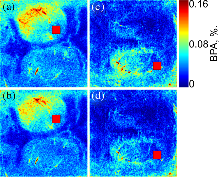

In order to compare the results of the CSD wave detection by LFP, BPI, and OIS techniques, we plotted in Fig. 8 time-traces of the BPA and CBV values spatially averaged within the ROI #1 ($20\times 20\text{pixels}$) centered with the place of KCl application together with the LFP traces. Due to the specific of animals’ preparation, the LFP electrodes were fixed to the skull outside the cranial window. Consequently, an additional time was needed for the neuronal component (measured by LFP) to cover the distance between the ROI #1 and the recording electrode. Assuming that the speed of the CBV component is about the same as the speed of the neuronal component measured by LFP,^13,15,19 we can reconstruct the initial moment of the LFP-dip appearance at the place of the ROI #1. Such a reconstruction shows that the neuronal component always precedes both all vascular CSD components: the delay between the reconstructed LFP and constrictive CBV component (which always appears the first among vascular components, see Sec. 3.4) is in the range of 12 to 69 s.

Fig. 8

Time traces with primary and secondary CSD observed in BPI (blue lines), OIS (red lines), and LFP (black lines) for rat #1 (a) rat #3 (b), and rat #5 (c). BPI and OIS time-traces were evaluated in the ROI #1centered with the KCl application. The time scale of the LFP signal was recalculated to the position of ROI #1. Relative position in the time scale of signals extremes is indicated by the red and blue dashed lines for primary and secondary CSD events, respectively.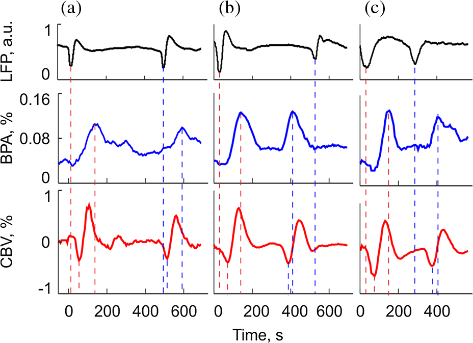

As seen in Fig. 8, the BPA component is always delayed with respect to the constrictive CBV component for both primary and secondary CSD waves. This delay varies for different animals in the range between 16 and 97 s. It may either increase from 46 s for the primary CSD event to 80 s for the secondary event in the rat #6 or decrease from 78 to 28 s in rat #5, or show small changes (from 84 to 97 s) in rat #1. Note that during the secondary CSD event in rat #3 [Fig. 8(b)], all vascular components appear 260 s earlier than the LFP signal. The situation is opposite for the secondary event in rat #5 where the constrictive CBV component is delayed with respect to the LFP dib by 160 s, while in rat #1, the LFP and constrictive CBV waves appear simultaneously.