2.1.

TIR-Cerulean Fusion Protein and Acceptor-Labeled Decoy Peptides

Expression vectors that encode TLR4 and TLR2 fused with Cerulean fluorescent protein were described previously.¹⁸ Cell-permeating decoy peptide 4BB used in this study was previously identified as potent TLR4 inhibitor that binds the TIR domain of TLR4.¹⁸ 4BB decoy TIR-derived sequence was amended by the cell-permeating Antennapedia homeodomain sequence¹⁹ placed at the N-terminus. 4BB peptide was labeled with Bodipy TMRX (BTX) N-terminally. Peptide synthesis, labeling, and verification were performed at the University of Maryland Biopolymer-Genomics Core Facility as previously described.¹⁸

2.2.

Fluorescence Lifetime Imaging Microscopy

Fluorescence lifetime images were acquired using FLIM system (Alba 5 from ISS). The excitation was from laser diode 443 nm coupled with scanning module (ISS) through multiband dichroic filter $443/532/635\mathrm{nm}$ (Semrock) to microscope (Olympus IX71S) with objective $20\times 0.45\mathrm{NA}$ (UPlan Olympus, Center Valley, Pennsylvania). Emission was observed through bandpass filter $480/30\mathrm{nm}$ (Chroma Technology, Bellows Falls, Vermont) and detected by a photomultiplier H7422-40 (Hamamatsu). FLIM data were acquired using FD modality (ISS A320 FastFLIM electronics) with $n$ harmonics of 20 MHz laser repetition frequency ($n=1$, 2, 3, 4, 5, 6). FastFLIM was calibrated using fluorescein in buffer pH 8.0 as a standard with single lifetime of 4.0 ns. Images were acquired using the following setting: image size of $256\times 256\text{pixels}$, scan speed $1\mathrm{ms}/\text{pixel}$ (or about $1\mu \text{m}/\text{pixel}$) with two to five overlapping scans. FLIM data were analyzed with VistaVision Suite software (Vista v.204 from ISS).

2.3.

Visualization of FD FLIM Data with Phasor Plot

Single- or multifrequency FLIM images were mapped into phasor plots using VistaVision Suite software (Vista v.204 from ISS). Briefly, each pixel in the FLIM image is represented as a point in the two-dimensional (2-D) polar plot with coordinate $S$ and $G$ based on the measured phase shift ($\phi$) and demodulation factor ($m$). For single exponential lifetime FLIM data, the phasor plot is represented by points located at half circle, which represents all possible single exponential lifetimes related to the coordinate $S(0,1)$ and $G(0,0.5)$ values as

In case of FLIM data with multiexponential lifetimes, the points in the phasor plot are the results of superposition of single lifetimes. The positions of points are inside the semicircle and follow vector algebra. For biexponential decays, the possible locations of the points are along the line joining the two lifetime points defined by the fractional contribution of each component ($f_i$) in the observed total intensity as

A detailed description of the principles of the phasor plot can be found elsewhere.^20–24

2.4.

Lifetime Background Correction

Multifrequency FLIM data were corrected for contribution of background fluorescence from cell autofluorescence using VistaVision Suite software v. 204 from ISS. The principle of correction is based on the phasor plot concept. Because points on the phasor plot are generated based on the composition of vectors of each individual fluorescing species, vector algebra can be used and the unwanted component can be subtracted regardless of its intensity decay complexity. Detailed analytical procedure for lifetime background correction is provided in Sec. 3.2. Some procedures for correcting FD lifetime data were already developed for single point measurements.^25,26

2.5.

Lifetime Data Analysis

Multifrequency FLIM data were analyzed with VistaVision Suite software using single- and biexponential intensity decay models and nonlinear error-weighted fit. Lifetime fitting was performed using binned pixels and fixed errors for phase and modulation (0.4 deg and 0.01) for each frequency. Average lifetime images were generated based on pixel-by-pixel analysis using combined intensity of two neighboring pixels in all direction ($\mathrm{bin}2=25\text{pixels}$). The binning was necessary because of usually weak intensity of single pixels. For multiexponential decays, the average lifetimes are calculated from fitted parameters, decay times ${\tau }_i$ and amplitudes ${\alpha }_i$ (or fractional intensities $f_i$)²⁷

VistaVision Suite software provides capability for displaying images for each of the calculated decay time parameters.

For calculation of FRET efficiency, amplitude-weighted average lifetimes of donor alone, ${\tau }_{\mathrm{D}}$ and donor-acceptor pair ${\tau }_{\mathrm{DA}}$ should be used if the intensity decay is nonsingle lifetime

This is because the unquenched and quenched donors display the same radiative decay rate and the change in lifetime is proportional to change in quantum yield. The above discussion is valid for FRET systems when all donor molecules are affected by acceptor molecules. This applies to DA pairs at unique distances, DA pairs with distance distribution, and for homogeneous spatial distribution of donor and acceptor molecules (e.g., solutions). In biological systems, in particular protein-protein interaction studies, it is very difficult (or even impossible) to fulfill the conditions that all donor-labeled proteins undergo interaction with acceptor-labeled proteins. Low binding affinity between donor- and acceptor-labeled biomolecules and limited acceptor concentration results in the presence of significant amounts of free, noninteracting donor molecules, thereby making it difficult to determine the exact value of ${\tau }_{\mathrm{DA}}$. Therefore, the FRET efficiency calculated based on Eq. (6) reflects, in most cases, an apparent value which is qualitative indication of a protein-protein interaction.

3.1.

Visualization of Intensity Decays of Cerulean Fused Proteins with Phasor Plot

The phasor plot is a graphical representation of intensity decays for an FLIM image. Point positions in the 2-D phasor plot are defined by the values of sine ($S$) and cosine transform ($G$) given by Eqs. (1)–(3). FD FLIM images contain information on the phase shift ($\phi$), DC, and AC intensities for each pixel of the image and for each modulation frequency ($f$). Therefore, the phasor plot can be displayed even during data acquisition. The DC and AC values are used for calculation of modulation ($m$). Experimental data that illustrate the single- and biexponential intensity decays are presented in Figs. 1 and 2, respectively. An image of the HeLa cells transfected with TLR2-Cer fusion protein and multifrequency phasor plot is shown in Fig. 1. For each modulation frequency, the points form a single round cluster located at the semicircle of the phasor plot. Such a location indicates that TLR2-Cer fluorescence decay is single exponential, and the lifetime value can be determined using Eq. (1).

Fig. 1

Multifrequency phasor plot of a single-exponential decay. (a) Fluorescence intensity image of HeLa cells transfected with TLR2-Cer. (b) Corresponding multifrequency phasor plot is shown for the frequencies of 20, 40, 60, 80, 100, and 120 MHz (counter clockwise). (c) The area highlighted in purple corresponds to the points selected by a circle on the phasor plot and has single-exponential lifetime of about 2.8 ns. Image was processed using VistaVision Suite software v. 204 from ISS.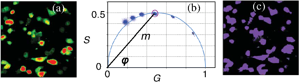

Fig. 2

(a) Multifrequency phasor plot for biexponential fluorescence decay characteristic for images of HeLa cells transfected with TLR4-Cer in the presence of peptide 4BB-BTX. The modulation frequencies are 20, 40, 60, and 100 MHz (counter clockwise). (b) The area highlighted in purple on the FLIM image corresponds to the cluster of points selected with the circle on the phasor plot that have predominantly single exponential lifetime of $\sim 2.8\mathrm{ns}$. (c) Interpretation of a biexponential phasor plot.

The phasor plot can be used in reverse mode so that the points selected on the plot with a cursor are highlighted in the DC image [Fig. 1(c)]. This procedure enables the identification of fluorescent species with specified lifetimes and was successfully used in complex cellular system.²² Because TLR2-Cer has a single lifetime, all pixels that correspond to fluorescent cells are uniformly highlighted in the DC image despite high intensity heterogeneity between individual cells (more than two orders of magnitude). Lifetime data analysis for a fluorophore with a single lifetime component is straightforward and does not require the fitting procedure. Even though a multifrequency phasor plot was generated, a single modulation frequency is sufficient to determine the lifetime value according to Eq. (1). Calculations indicate that the uniform lifetime has a value of $\sim 2.8\mathrm{ns}$ across the image.

We previously demonstrated that a decoy peptide derived from the dimerization interface of TLR4 TIR domain, 4BB, strongly binds TLR4 TIR.¹⁸ Therefore, when HeLa cells are transfected with TLR4-Cer fusion protein and incubated with 4BB-BTX, FRET was anticipated and the corresponding phasor plot should reflect multiexponential intensity decay (Fig. 2). For each modulation frequency, the observed linear distribution of points on the phasor plot indicates that intensity can be interpreted as biexponential. Two distinct lifetime components and their various fractional intensities can be determined from the phasor plot using single frequency [Fig. 2(c), see also Eqs. (2) and (3)].²⁰ Cluster of points located on the semicircle represents the single lifetime similar in value to that observed for TLR2-Cer of 2.8 ns [compare Figs. 2(a) and 1(b)]. Cells that displays long lifetime of $\sim 2.8\mathrm{ns}$ are highlighted indicating unquenched or minimally quenched donor. Not highlighted areas are related to the points on the phasor plot that display shorter nonsingle lifetimes, thus indicating measurable FRET.

It should be noted that distribution of points on the phasor plot for multiexponential intensity decay depends on the modulation frequency. Phasor plots of real FLIM images always display as diffusive spots because of noise in the system. A common and primary source of the noise are related to image pixels with weak emission.²⁸ Phasor plots for TLR2-Cer (Fig. 1) are significantly less noisy than for TLR4-Cer/4BB-BTX (Fig. 2) for each modulation frequency. This observation is in agreement with the difference in pixel intensities, as TLR2-Cer displays about 10-fold higher intensities compared to the TLR4-Cer. The observed increased noise for phasors with increased frequencies is related to properties of our multifrequency FLIM system. At 20 MHz frequency, our system has an apparent modulation depth of about 1.7 which decreases by $\sim 5$-fold at 120 MHz. The loss of modulation depth due to signal processing and detector response is the reason of larger phasor noise at higher modulation frequencies. The origin of observed small deviations of points outside the semicircle for higher frequencies is not known. We think that this may be due to difference in procedure used for calibration (emission window $525/30\mathrm{nm}$ for fluorescein with 4 ns) and Cer imaging ($485/30\mathrm{nm}$). We choose 60 MHz frequency for phasor analysis, however, similar analysis at 40 or 80 MHz would give similar results.

3.2.

Background Correction of FLIM Data

The concept for background correction is shown in Fig. 3(a), where the observed vector $R_{\mathrm{O}}$ is a composition of fluorophore $R_{\mathrm{F}}$ and background $R_{\mathrm{B}}$ vectors

Fig. 3

Concept for background correction based on phasor plot. (a) Vector representation of background fluorescence ${\mathbf{R}}_{\mathrm{B}}$, raw observed or measured ${\mathbf{R}}_{\mathrm{O}}$, and corrected fluorescence ${\mathbf{R}}_{\mathrm{F}}$ vectors. (b) Corrected $S$ and $G$ coordinates for three observed vectors (${\mathbf{R}}_1$, ${\mathbf{R}}_2$, ${\mathbf{R}}_3$) calculated for background contribution increasing from 0.1 to 0.5 (red circles).

Given that parameters of background vector $(m_{\mathrm{B}},{\phi }_{\mathrm{B}})$ are known, each observed pixel parameters $(m_{\mathrm{O}},{\phi }_{\mathrm{O}})$ can be corrected for background contribution $f_{\mathrm{B}}$ ($f_{\mathrm{B}}=I_{\mathrm{B}}/I_{\mathrm{O}}$, where $I_{\mathrm{B}}$ and $I_{\mathrm{O}}$ are the intensities of background and observed pixels, respectively). Examples of background correction effects are shown in Fig. 3(b) for three different vectors. Vector (1) display longer lifetime, vector (2) is collinear, and vector (3) display shorter lifetime compared to the background. Calculated points (red circles) represent the various background contributions, $f_{\mathrm{B}}=0.1$, 0.2, 0.3, 0.4, 0.5. The important observation is that corrected points ($S_{\mathrm{F}}$, $G_{\mathrm{F}}$ coordinates) will be on the line connecting observed and background vectors. This is a consequence of phasor linearity and is independent of the complexity of intensity decays of both vectors. The linearity of phasor coordinates allows all background components (cell autofluorescence, signal from sample matrix, scattered excitation component, etc.) be included into one background vector specific for particular modulation frequency. If the applied background contribution exceeds its real value, the corrected points on the phasor plot may be placed outside the semicircle (see corrected points for vector ${\mathbf{R}}_1$ with $f_{\mathrm{B}}>0.4$). Such positions would indicate that intensity decay contains negative pre-exponential factor. In the case when intensity decay of acceptor is observed, the appearance of phasors outside the semicircle indicates that acceptor emission is from FRET excitation. Such a resolution of acceptor emission from direct excitation and via FRET is discussed in details elsewhere.²⁹

Raw FLIM data for the FRET system of TLR4-Cer/4BB-BTX are shown in Fig. 4(a). The brightness of TLR4-Cer fluorescence in individual cells varies widely across the image. It is important to note that a transient transfection of an exogenous gene to a cell line typically produces a cell population highly heterogeneous with respect to the level of transgene expression in individual cells, with some cells in the population not expressing the exogenous gene at all.

Fig. 4

Phasor plot based selection of image area for background correction. Image areas highlighted in blue color in the right panel corresponds to the points selected by circle in phasor plot (middle panel). (a) FLIM image of cells transfected with TLR4-Cer and treated with acceptor 4BB-BTX (50 μM) and (b) untransfected cells treated with acceptor. Phasor plots are displayed at modulation frequency of 60 MHz for pixels with intensity below 30 counts.

Intensity decay of cell autofluorescence is intrinsically multicomponent which depends on cell metabolic state, and excitation and observation spectral windows.³⁰ Thus, the background fluorescence parameters has to be determined specifically in the cellular system under investigation, using a control image of cells that do not express donor. In a hypothetical case, when all cells would express donor, the background fluorescence parameters should be determined from a control image of not transfected cells, as shown in Fig. 4(b). In this work, however, we took advantage of the fact that not all cells in our images express Cer donor and used signal from dim cells to calibrate the background correction. We also assumed that autofluorescence intensity and lifetime composition is homogeneous across the entire image. Narrow emission range of $485/30\mathrm{nm}$ was used. The selection of dim cells for background correction was justified by comparison of phasor plots of raw FLIM data for FRET system and control sample with cells not transfected with TLR4-Cer (Fig. 4). The diffusive character of phasor plots shown in Fig. 4 originates from pixels that have low intensity. The correction background phasor vector is taken as an average over many pixels from selected image area highlighted with blue color [Fig. 4(a)]. The use of the same image for the identification of background parameters and for the FRET analysis is advantageous because potential biases due to the difference in biochemical procedures, in sample matrix, and in instrumental setup are not present. The background signal from dim cells originates mostly from cell autofluorescence. The signal from sample matrix (areas between cells) contributes $<10\%$ to the total background signal. Background vector parameters ($m_{\mathrm{B}}$ and ${\phi }_{\mathrm{B}}$) for each modulation frequency are shown in Fig. 5. By fitting multifrequency FLIM data to biexponential model, the background decay times were estimated as 0.85 and 4.2 ns and fractional intensities of 0.516 and 0.484, respectively.

Fig. 5

Multifrequency FLIM data for background correction. Lines show fit to biexponential decay model.

Phasor plot of corrected FLIM image is shown in Fig. 6 along with that of the raw image and the image with applied intensity threshold. In order to facilitate direct comparison of the phasors, the intensity threshold was set to 60 counts resulting in the same number of processed pixels. Phasor plot for raw data displays broadly the distributed points that include a mixture of signals from background and donor. As shown in Fig. 4(a), the majority of points originate from dim cells identified as background fluorescence. In the conventional FLIM approach, low intensity cells are removed from the analysis by applying an intensity threshold. This approach is satisfactory if the background contribution is low. However, in FRET systems one expects that quenched donor may display low intensity and removal of less bright cells may limit information on FRET. Removal of pixels with intensities below 60 counts/ms (twice of the background average signal) resulted in a simpler phasor plot with linear shape that suggests biexponential intensity decay [Fig. 6(b)]. It is important to note that the intensity threshold procedure limits the image to the brighter cells which may display simpler intensity decay, however, the position of points in the phasor plot remains unchanged.

Fig. 6

Effect of background correction on FLIM data presented in Fig. 4(a). Phasor plots at 60 MHz for (a) the raw FLIM image [see Fig. 4(a)], (b) raw image with intensity threshold above 60 counts, (c) background corrected image with intensity threshold of 30 counts. Average background intensity was 30 counts.

The phasor plot for background corrected FLIM data [Fig. 6(c)] is significantly different compared to that produced by the intensity threshold procedure [Fig. 6(b)]. Every pixel in the image is corrected according to the procedure described by Eqs. (8) and (9), thus resulting in a change of point positions according to the contribution of background at each pixel as illustrated in Fig. 3(b). Background correction was applied with an average intensity of 30 counts and phasor displayed for pixels with intensities above 30 counts. Some points were moved outside the semicircle which implies that the background contribution for those pixels is likely overestimated. This is the result of using uniform background signal which, in fact, also slightly varies. Such background correction artifacts are difficult to avoid when working with a highly heterogeneous cell population. For simplicity, correction of the FLIM data is shown only for 60 MHz modulation frequency, however data at other frequencies (20, 40, 80, 100, and 120 MHz) were corrected simultaneously (see background parameters in Fig. 5). Overall, the background correction not only removes the undesired decay components but also leads to significantly simplified lifetime analysis of FLIM data. For TLR4-Cer/4BB-BTX FRET system that display multicomponent raw FLIM data, this procedure reduces complexity to a biexponential model.

In the FRET studies, the same correction procedure should be performed for donor in the absence of the acceptor. The corrected FLIM data for TLR4-Cer transfected to HeLa cells are shown in Fig. 7. Earlier, we demonstrated that TLR2-Cer displays a single lifetime (Fig. 1). We also observed that HeLa cells transfected with Cerulean not fused to a TIR domain also display a single lifetime (data not shown). However, when Cerulean is fused with TLR4 and expressed in HeLa cells, the fluorescence decay becomes nonsingle exponential. The points on the phasor plot for donor alone, TLR4-Cer, can be approximated using a biexponential model with lifetimes 2.85 and 0.75 ns (Fig. 7, dashed line). The contribution of the short component is low as indicated by the location of the majority of points at the upper part of the phasor plot. This lifetime heterogeneity may be a consequence of the ability of TLR4 to dimerize. The heterogeneous behavior of TLR4-Cer was observed even for bright cells which imply that this is not an artifact of background correction. The nonsingle exponential decay of donor usually complicates the quantitative analysis of FLIM FRET data. The mechanisms of lifetime heterogeneity characteristic for some fluorescent proteins are not yet clear. The underlying reasons for this heterogeneity have been associated with different forms of chromophores,^3,13,16 homodimerization of fused proteins that can lead to energy homotransfer^1,31 as well as the effect of photobleaching.^32,33 Some effect of photobleaching on the heterogeneity of TLR4-Cer cannot be completely excluded at this time. Because of the weak expression of TLR4-Cer, higher laser excitation was used that might cause 5% to 10% photobleaching during image acquisition.

Fig. 7

Intensity image and phasor plot of background-corrected FLIM data for TLR4-Cer in the absence of acceptors. Data correspond to the 60 MHz modulation frequency.

3.3.

FLIM FRET Analysis Using Phasor Plot and Multifrequency Phase-Modulation Data

When the donor displays single exponential decay in the absence and presence of acceptor, phasor plots will have two clusters of points (assuming spatial separation between cells with and without FRET) that identify lifetimes of free donor and donor bound to acceptor, ${\tau }_{\mathrm{D}}$ and ${\tau }_{\mathrm{DA}}$. As mentioned previously, such a distribution is rarely observed in cellular systems for images that include many cells. In the TLR4-Cer/4BB-BTX system, the positions of points in the phasor plot are scattered along an imaginary line [Fig. 6(c)]. By applying the principles of phasor linearity shown in Fig. 2(c), ${\tau }_{\mathrm{D}}$ and ${\tau }_{\mathrm{DA}}$ can be identified graphically by plotting an imaginary line along the points and finding the values of ${\tau }_{\mathrm{D}}$ and ${\tau }_{\mathrm{DA}}$ at the intersection of the line and semicircle. The estimated lifetimes are ${\tau }_{\mathrm{D}}=2.85\mathrm{ns}$ and ${\tau }_{\mathrm{DA}}=0.65\mathrm{ns}$ resulting in an FRET efficiency of $E=0.77$ for donor-acceptor pairs ($E=1-{\tau }_{\mathrm{DA}}/{\tau }_{\mathrm{D}}$). The spread of points between 2.85 and 0.65 ns lifetimes indicates that the substantial number of pixels is the mixture of unquenched donor and donor acceptor pairs. Assuming that the intensity decay is approximated with biexponential model, decay times, and amplitudes (or fractional intensities) of each component can be determined. Using unconstrained biexponential model, the resulting decay time parameters usually vary significantly from pixel to pixel and may have no meaningful values as individual numbers. This is a consequence of a correlation between fractional intensities (or amplitudes) and decay times, and frequent presence of pixels with weak signals. Pixel-by-pixel biexponential fitting analysis of FLIM data for the TLR4-Cer/4BB-BTX FRET system in HeLa cells is displayed as an average lifetime image and a histogram of lifetime distribution in Fig. 8. There is a dramatic difference in results of lifetime analysis for the background corrected and uncorrected data. Despite a simple phasor plot [Fig. 6(b)], the average lifetime for uncorrected data is substantially affected by cell autofluorescence and it is difficult to conclude on FRET because of broad lifetime distribution. Data corrected with lifetime background display well defined peaks with the average lifetime of 0.75 and 2.85 ns and substantially rearranged lifetime distribution that reflects the mixture of unquenched and quenched donors. The pixel frequency at peak with 2.85 ns lifetime is much larger than for uncorrected data which reflects the effect of background correction when low donor expressed and no FRET cells contribute to this peak. The peak with short average lifetime of 0.75 ns cannot be regarded as single lifetime but is related to cells with dominant DA complexes. This is because the phasor plot shown in Fig. 6(c) displays cluster of points, which are off the semicircle at lower part of the plot.

Fig. 8

Lifetime analysis of TLR4-Cer fluorescence in HeLa cells in the presence of acceptor 4BB-BTX using raw (a) and background corrected (b) FLIM data. Average lifetime images (amplitude weighted) are displayed as histograms (left) and in pseudocolor images (right) with values from 0 to 3.5 ns. Nonlinear fitting of multifrequency FLIM data was performed with binning ($\mathrm{bin}2=25\text{pixels}$) with fixed errors of phase of 0.4 deg and modulation of 0.015 and no constrains on decay and amplitude values.

Typically, a biexponential fit of FLIM data is substantially more reliable when some fitting constraints applied. Using two spatially invariant lifetimes, ${\tau }_{\mathrm{D}}=2.85\mathrm{ns}$ and ${\tau }_{\mathrm{DA}}=0.65\mathrm{ns}$, normalized amplitudes (${\alpha }_{\mathrm{DA}}=1-{\alpha }_{\mathrm{D}}$) for each component can be obtained at each pixel. Because unquenched and quenched TLR4-Cer have the same radiative decay rate but different nonradiative rates, the amplitudes can be interpreted as relative molecular concentrations of [D] and [DA]. Results of such an FLIM FRET analysis are shown in Fig. 9. A significant difference is observed for uncorrected and corrected FLIM images. The molecular fraction of [DA] varies between cells as well as within single cells. Analysis using uncorrected data leads to substantially overestimated contribution of [DA] pairs. These results demonstrate that the background correction allows for quantitative analysis of FLIM FRET data for heterogeneous population of cells. Further data processing can reveal the information on the association constant of [DA] complex. Because amplitudes are proportional to molecular concentration of noninteracting [D] and interacting donor [DA], it is possible to estimate the binding affinity between the interacting biomolecules according to

Fig. 9

Analysis of FRET system TLR4-Cer/4BB-BTX in HeLa cells using FLIM FRET. Fraction of donor-acceptor pairs is presented as histogram (left) and in pseudocolor scale from 0 to 1.0 (right) for uncorrected (a) and background corrected FLIM data (b). Nonlinear fitting of multifrequency FLIM data was performed with binning ($\mathrm{bin}2=25\text{pixels}$) with fixed errors of phase of 0.4 deg and modulation of 0.015 and fixed lifetime components of 2.85 ns (donor) and 0.65 ns (donor-acceptor pair).

Fig. 10

Normalized amplitude ratio distribution in FLIM images of TLR4-Cer-expressing HeLa cells incubated without (dashed line) and in the presence of 4BB-BTX for 1 h (solid line). FLIM data were fitted using biexponential model with two fixed lifetimes of 2.85 and 0.65 ns.