Enhanced spatial resolution in fluorescence molecular tomography using restarted L1-regularized nonlinear conjugate gradient algorithm

Junwei Shi; Fei Liu; Guanglei Zhang; Jianwen Luo; Jing Bai

doi:10.1117/1.JBO.19.4.046018

28 April 2014 Enhanced spatial resolution in fluorescence molecular tomography using restarted L1-regularized nonlinear conjugate gradient algorithm

Junwei Shi, Fei Liu, Guanglei Zhang, Jianwen Luo, Jing Bai

Author Affiliations +

Journal of Biomedical Optics, Vol. 19, Issue 4, 046018 (April 2014). https://doi.org/10.1117/1.JBO.19.4.046018

Abstract

Owing to the high degree of scattering of light through tissues, the ill-posedness of fluorescence molecular tomography (FMT) inverse problem causes relatively low spatial resolution in the reconstruction results. Unlike L2 regularization, L1 regularization can preserve the details and reduce the noise effectively. Reconstruction is obtained through a restarted L1 regularization-based nonlinear conjugate gradient (re-L1-NCG) algorithm, which has been proven to be able to increase the computational speed with low memory consumption. The algorithm consists of inner and outer iterations. In the inner iteration, L1-NCG is used to obtain the L1-regularized results. In the outer iteration, the restarted strategy is used to increase the convergence speed of L1-NCG. To demonstrate the performance of re-L1-NCG in terms of spatial resolution, simulation and physical phantom studies with fluorescent targets located with different edge-to-edge distances were carried out. The reconstruction results show that the re-L1-NCG algorithm has the ability to resolve targets with an edge-to-edge distance of 0.1 cm at a depth of 1.5 cm, which is a significant improvement for FMT.

1. Introduction

As a promising low-cost and noninvasive molecular imaging modality profiting from the availability of a variety of highly specific fluorescent molecular probes, fluorescence molecular tomography (FMT) has been applied for detection and follow-up of tumor growths, cell trafficking, immune and treatment responses, and is expected to find further applications in biomedical research and drug discovery.¹^–⁶ By detecting the photon density over the animal surface, FMT can offer three-dimensional (3-D) and quantitative visualization of fluorescence distribution in small animals in vivo.

However, only with the photon distribution measured at the surface, the reconstruction of FMT is an ill-conditioned problem due to the high degree of scattering of photons propagating through tissues. This accordingly incurs a poor spatial resolution in FMT, which is an important technical challenge. Even though more fluorescence information can be captured by multispectral technique⁷^–¹⁰ or multiple spatial patterns of illumination,¹¹^–¹⁴ the FMT inverse problem is still ill-conditioned and consumes much time and memory. Moreover, the reconstruction of FMT is highly susceptible to noise and numerical errors. To compute a meaningful approximate solution, penalty terms are typically incorporated into the regularization function. For example, regularization functions are chosen to enforce smoothness,¹⁵ promote sparsity,¹⁶^–¹⁸ or incorporate anatomical information.¹⁹^–²¹ In addition, based on compressed sensing, some convex optimal algorithms have been used in the FMT inverse problem.²²^–²⁵ Among these, quadratic penalty (i.e., L2 regularization) is commonly used since it is simple and can be efficiently solved by a large range of standard minimization algorithms, such as the Tikhonov method. However, the fast spatial changes in the solution are often oversmoothed, and the localized features are lost during the reconstruction process.¹⁶ Unlike L2 regularization, L1 regularization can preserve details, such as edges and smooth out noise, especially when the reconstructed fluorophore distribution is sparse. Recently, we proposed an efficient restarted L1 regularization-based nonlinear conjugate gradient (re-L1-NCG) algorithm for FMT reconstruction, which can increase the computational speed with low memory consumption and high localization accuracy.²⁶

From the aspect of algorithm design, a key issue is how to design an algorithm to obtain the reconstruction results with high spatial resolution. Plenty of efforts have been donated to improve the spatial resolution of FMT by separating fluorescent targets with small edge-to-edge distance (EED).²¹^,²⁷^–³⁰ By taking advantage of the different variation trends of fluorescence yields caused by kinetic concentration or multispectral excitation, principal component analysis was used to resolve fluorophores neighboring each other closely.²⁷^,²⁸ In the multimodality imaging system combining positron emission tomography (PET) and FMT, the target prior information from PET images was employed in the FMT reconstruction procedure using the iteratively reweighted least-squares method, and improved spatial resolution was observed.²¹ In addition, time-resolved measurement of early arriving photons has been demonstrated by a number of groups to reduce photon scatter, which contributes to improving the spatial resolution effectively.²⁹^,³⁰ However, it should be noted that these aforementioned reconstruction methods rely on some auxiliary means, such as kinetic concentration, multispectral excitation, prior information from anatomy images, and early photons. These methods cause long data-collection interval or require additional anatomical information for the reconstructed targets, which will decrease the reconstruction speed and consume much memory. Thus, it is very necessary to design a reconstruction method that can improve the spatial resolution of FMT without any auxiliary information. In this paper, the previously proposed re-L1-NCG algorithm is adopted to obtain high spatial resolution in FMT.

In re-L1-NCG, the NCG algorithm with backtracking line search (BLS) is used to solve the L1 regularization optimization problem,³¹ which is abbreviated as L1-NCG. However, the convergence speed of L1-NCG decreases after some iterations due to the ill-condition of FMT inverse problem. In order to increase the convergence speed, we proposed a restarted strategy in which the searching descent direction and the permission domain would be reset after a fixed number of iterations. It should be noted that the permission domain in this paper is obtained using L1-NCG without additional anatomical information. In order to compensate for the low level of emission light coming from nodes deep in the tissue, the pretreatment is carried out by normalizing the columns of system matrix of FMT problem. For comparison, Tikhonov (a conventional L2-regularized method) and L1-Ls (a well-known L1-regularized method) are adopted. Through adding logarithmic barrier penalties, L1-Ls obtains the optimal point by a specialized interior-point method using the preconditioned conjugate gradients (PCG) algorithm to compute the search direction.³² In simulation and physical phantom studies, double fluorescent targets with different EEDs (0.1 to 0.6 cm) at a depth of 1.5 cm are employed to evaluate the performance of different reconstruction methods in terms of spatial resolution.

This paper is organized as follows. In Sec. 2, the mathematical framework of FMT and the re-L1-NCG algorithm are presented, and a merit function is proposed to quantitatively analyze the spatial resolution. In Sec. 3, numerical simulations and physical phantom studies are conducted to validate the enhanced spatial resolution in the reconstruction results using the proposed algorithm. The results are discussed and this paper is concluded in Sec. 4.

2. Method

2.1.

Model of Diffusion Equation

To solve the forward problem is to predict the values of the observable measurements, according to the distribution of fluorochrome and other model parameters. Considering the computational burden of the radiative transfer equation (RTE), the forward model used to predict photon propagation in highly scattering media is based on the coupled diffusion equations (DE) with Robin-type boundary condition.³³ In practice, absolute experimental measurements cannot be acquired since it is nearly impossible to accurately measure the incident light intensity and the corresponding instrumentation response functions. Consequently, referencing approaches should be adopted.³⁴ Through the normalized Born approximation to the DE, the nonlinear FMT problem can be linearized and all the position-dependent gain factors in the forward model can be canceled out.³⁴^,³⁵ The normalized Born average intensity at location $r_{d}$ corresponding to an illumination spot located at $r_{s}$ can be formulated as follows:

Eq. (1)

ϕ_{f} (r_{d}, r_{s}) = \frac{ϕ_{em} (r_{d}, r_{s})}{ϕ_{ex} (r_{d}, r_{s})},

where

ϕ_{em} (r_{d}, r_{s})

denotes the average intensity at emission wavelength

λ_{2}

and

ϕ_{ex} (r_{d}, r_{s})

denotes the average intensity at excitation wavelength

λ_{1}

. Then the normalized Born approximation can be formulated as follows:

Eq. (2)

ϕ_{f} (r_{d}, r_{s}) = \frac{S_{0} υ}{G (r_{s}, r_{d}, λ_{1}) D^{f}} \int G (r_{d}, r, λ_{2}) x (r) G (r_{s}, r, λ_{1}) d^{3} r,

where

G (r_{s}, r, λ_{1})

denotes the analytically calculated photon field at excitation wavelength

λ_{1}

induced at position

r

by a source at position

r_{s}

in the tissue.

G (r_{d}, r, λ_{2})

is the Green’s function, which describes photon propagation from point

r

to the detector point

r_{d}

at emission wavelength

λ_{2}

.

D^{f}

is the diffusion coefficient of tissue at emission wavelength

λ_{2}

,

υ

is the speed of light in the tissue, and

S_{0}

is a calibration factor accounting for various system gain and attenuation factors. Kirchhoff approximation (KA) as an analytical method is used to solve the FMT forward model, in order to ease the computational burden of numerical methods (such as the finite element method).³⁶ After the image domain is discretized, the FMT problem can be formulated as the following linear matrix equation:

Eq. (3)

Φ_{f} = W X,

where

W

denotes the weight matrix (or sensitive matrix) mapping the unknown vector of fluorochrome concentrations (

X

) into the measured surface fluorescence vector (

Φ_{f}

). Detailed descriptions can be found elsewhere.³⁵

2.2.

FMT Reconstruction Based on L1 Regularization

Through DE forward model, Eq. (3) couples the fluorochrome distribution ( $X$ ) to the measurements ( $Φ_{f}$ ) with the weight matrix $W$ . To solve the inverse problem of FMT is to infer the distribution of fluorochrome ( $X$ ) from the measured values of the observable measurements ( $Φ_{f}$ ). The inverse problem can be directly solved by inverting the weight matrix $W$ . However, this inversion is often ill-posed in the Hadamard sense, as the dimension of the null space of $W$ is not zero. To guarantee the uniqueness and stability of FMT inverse problem and to preserve high spatial resolution, L1 regularization is adopted.²⁶ For the FMT inverse problem, the optimization function is formulated as follows:

Eq. (4)

\underset{X \geq 0}{\arg \min} {‖ W X - Φ_{f} ‖}_{2}^{2} + λ {‖ X ‖}_{1},

where

λ

is the regularization parameter balancing the data fitting and L1 penalty. Through normalizing the columns of matrix

W

defined in Eq. (3), the high attenuation of emission light coming from deep fluorochromes in the tissue can be compensated.³⁷ By means of normalization, the resultant preconditioned optimization function is rewritten as follows:

Eq. (5)

X_{L 1} = \underset{X \geq 0}{\arg \min} [f (X) = {‖ W_{new} X - Φ_{f new} ‖}_{2}^{2} + λ {‖ X ‖}_{1}],

Eq. (6)

W_{nor} (i, j) = {\begin{matrix} {‖ W_{i} ‖}_{2}^{- 1} & i = j \\ 0 & i \neq j \end{matrix},

Eq. (7)

W_{new} = W W_{nor}; Φ_{f new} = Φ_{f} / \max (Φ_{f}),

where

W_{i}

is the

i

’th column of matrix

W

.

Equation (5) is solved through the NCG descent algorithm with BLS. NCG methods are well known in unconstrained optimization problems. However, it can be seen that Eq. (5) is constrained with non-negativity constraint. Although there are many methods to deal with the non-negativity constraint, such as logarithmic barrier penalties, alternating direction method of multipliers (ADMM), split Bregman, and proximal method, they seem a bit complicated compared with L1-NCG because they proceed by iteratively updating the primal and dual variables.¹⁶^,³⁸^,³⁹ In this paper, Eq. (5) is first computed by L1-NCG without non-negativity constraint. Then the negative values are set to zero. The detailed description of L1-NCG can be found elsewhere.²⁶^,³¹ As mentioned in Ref. 26, the search directions in the L1-NCG method are not strictly conjugative between each other, and the step lengths are approximated suboptimally, unlike in the linear conjugate gradient method. In addition, the severe ill-posedness of the FMT inverse problem makes it difficult to achieve satisfactory reconstruction results. Thus, restarted strategy is adopted to remit the aforementioned trouble of L1-NCG. In summary, the re-L1-NCG algorithm proposed in Ref. 26 is composed of inner iteration and outer iteration. When the search direction and initial value is set, the L1-NCG is applied in the inner iteration to get the sparse reconstruction results. Then based on the results reconstructed using L1-NCG, the permission region including the reconstructed fluorescent targets can be obtained. By resetting the search direction and the permission region, restarted strategy is realized in the outer iteration to increase the convergence speed of L1-NCG, which gives rise to satisfactory reconstruction results. The implementation of re-L1-NCG is summarized in Fig. 1.

Fig. 1

Flow chart of the restarted L1 regularization-based nonlinear conjugate gradient (re-L1-NCG) algorithm. $k_{inner}$ denotes the number of inner iterations of L1-NCG; $k_{outer}$ denotes the number of outer iterations; $k$ denotes the current number of the outer iteration.

When the number of iterations in L1-NCG is equal to $k_{inner}$ , the search direction for BLS is reset as negative gradient of $f (X)$ in Eq. (5).²⁶ After $k_{inner}$ iterations, the negative value in $X_{re - L 1}^{k}$ is set to zero, and then the new $X_{re - L 1}^{k}$ is used as the initial value for the next round of iterations because the performance of L1-NCG depends on the initial value. It is worth emphasizing that these nonzero positions in $X_{re - L 1}^{k}$ correspond to an approximate permission region, which includes the true fluorescent targets.²⁶ Then in matrix $W_{new}^{k}$ , the columns corresponding to zero in $X_{re - L 1}^{k}$ can be removed. Because the number of unknowns is dramatically reduced, the ill-posedness can be alleviated and the computational speed can be increased. Through the aforementioned permission region, the dimension of the matrix corresponding to Eq. (7) scales down sharply. This can increase the computational speed and reduce the memory consumption. After the first $k_{inner}$ inner iterations, the permission region is big enough to cover the true fluorescent targets. Along with the iteration, the size of the permission region gradually shrinks to the true size of the reconstructed fluorescent targets, until re-L1-NCG is terminated. By means of the L1 regularization combined with restarted strategy, reconstruction results with high spatial resolution can be obtained. It should be noted that one of the main roles of L1-NCG is to obtain an appropriate permission region for the restarted strategy. With the non-negative constraints, ADMM, proximal method, or split Bregman can obtain more accurate results, where the negative values do not appear in the reconstruction results.³⁸^,³⁹ However, in the frame of restarted strategy, these methods seem more complicated and need more time to obtain an appropriate permission region than L1-NCG.

When the cardinality of $X_{re - L 1}^{k}$ is smaller than a certain value (200) or the number of outer iterations exceeds the maximum (30), the re-L1-NCG algorithm is terminated. In addition, how to choose the regularization parameter under different experimental conditions is a difficult task, as the regularization parameter depends on the degree of ill-posedness. However, by adopting the normalization strategy shown in Eqs. (6) and (7), the reconstruction results with re-L1-NCG are not sensitive to the regularization parameter in a proper range. In this paper, the tuning parameters are manually optimized as described in Ref. 26, where $λ$ is set as 15.

In this paper, the Tikhonov method as a widely used analytical reconstruction method is adopted for comparison, and the suboptimal regularization parameter for Tikhonov is experientially selected based on $10^{- 5} \times tr (W W^{T})$ .⁴⁰ In addition, L1-Ls as an L1-regularized method is adopted to solve Eq. (4).³² In this paper, the optimal parameters of L1-Ls are set experientially. In L1-Ls, the regularization parameter is set to 0.00001; the maximum number of Newton iterations is set to 200; and the maximum number of BLS iterations is set to 100.

Actually, the spatial resolution of FMT system depends on several experimental parameters, including the wavelength of the emission light, the thickness of the tissues, the depth of the fluorescent targets, the arrangements of sources and detectors, the optical parameters, the reconstruction algorithms, the number of reconstructed fluorescence targets, etc.⁴¹^,⁴² The focus of this paper is the enhanced spatial resolution obtained using the re-L1-NCG algorithm. In this paper, two targets are separated with different EEDs in simulations and physical phantom experiments. In order to quantitatively analyze the performance of the algorithms in resolving the two targets, a relative merit function is defined as follows:⁴³

Eq. (8)

R = \frac{x_{\max}^{p} - x_{valley}^{p}}{x_{\max}^{p} - x_{\min}^{p}},

where

x^{p}

denotes the value of the profile along a given line on the reconstructed cross-section.

x_{\max}^{p}

and

x_{\min}^{p}

denote the maximal and minimal values of

x^{p}

, respectively.

x_{valley}^{p}

denotes the valley value between the two peak values corresponding to two targets. Thus,

R = 1

represents the highest spatial resolution and

R = 0

represents the lowest spatial resolution.

3. Experiments and Results

3.1.

Simulation Studies: Cylinder Model

Simulations are conducted to evaluate the performance of the re-L1-NCG algorithm. Figure 2 shows the geometry configuration of the simulations. A cylinder model was placed on a rotating stage, with the rotational axis defined as the $z$ axis and the bottom plane set as $z = 0 cm$ . The fluorophores were excited by a point source located at a height of $z = 0.75 cm$ . Fluorescence images of 360 deg full view were collected at every 10 deg (i.e., 36 projections were adopted). The numerical cylindrical phantom had a height of 1.5 cm and a diameter of 3 cm. Both fluorescent targets had a diameter of 0.4 cm and a height of 0.5 cm, and they were located at a depth of 1.5 cm with different EEDs ranging from 0.1 to 0.6 cm sequentially. In order to approximate high scattering media, the absorption coefficient and reduced scattering coefficient were set to 0.02 and $10 {cm}^{- 1}$ , respectively. The field of view (FOV) of the detector corresponding to each excitation source was $\sim 130 \deg$ , and the detector sampling distance was set to 0.2 cm. In order to simulate realistic situations, 5% Gaussian noise was added to the measurement data.

Fig. 2

Geometry configuration of the simulation study with double cylindrical fluorescent targets separated with different edge-to-edge distances (EEDs) (0.1, 0.2, 0.3, 0.4, 0.5, and 0.6 cm). The diameter of the cylindrical phantom is 3 cm, and the diameter of the cylindrical targets is 0.4 cm.

Through discretizing the geometry shown in Fig. 2, the linear matrix equation [Eq. (3)] was obtained using the KA method.³⁶ The size of the discrete elements was the same (0.13 cm) for cylindrical targets with different EEDs. By normalizing the system matrix and measurement data, the L1 regularization-based optimization function was constructed as Eq. (5). The reconstruction results obtained with the Tikhonov, L1-Ls, and re-L1-NCG algorithms are shown in Fig. 3, respectively. All the reconstructed images were normalized for better comparison. The small red circles in the slice images denote the real positions of the fluorescent targets. All the reconstruction results shown in Fig. 3 are taken from the $z = 1 cm$ plane. Different columns in Fig. 3 denote the reconstruction results for different EEDs. The first row of Fig. 3 denotes the reconstruction results obtained using the Tikhonov method. The results in the second and third rows of Fig. 3 are obtained using the L1-Ls and re-L1-NCG methods, respectively.

Fig. 3

Reconstructed fluorescent targets corresponding to different EEDs. The first, second, and third rows represent the cross-section reconstructed by Tikhonov, L1-Ls, and re-L1-NCG algorithms, respectively. The EEDs of the two fluorescent targets range from 0.1 to 0.6 cm.

As shown in Fig. 3, the reconstruction results obtained using the L1-Ls and re-L1-NCG methods have higher spatial resolution and signal-to-noise ratio than those obtained using the Tikhonov method. It can be seen in the first row of Fig. 3 that the two fluorescent targets reconstructed using the Tikhonov method can be distinguished when EED is $> 0.4 cm$ . When the EED is $< 0.3 cm$ , the fluorescent targets reconstructed using the Tikhonov method can hardly be distinguished. By contrast, the two fluorescent targets in the reconstruction results obtained with L1-Ls and re-L1-NCG can be distinguished, even when EED is 0.1 cm.

As a metric of the spatial resolution corresponding to different methods, the $R$ values calculated from Eq. (8) are listed in Table 1, and the $R$ value corresponds to the reconstructed cross-section profiles across the two targets at $x = 0$ (i.e., along the $y$ -axis direction) in Fig. 3. As shown in Table 1, the $R$ values corresponding to L1-Ls and re-L1-NCG are closer to 1, even when the EED is 0.1 or 0.2 cm. It means that the L1-Ls and re-L1-NCG methods can obtain higher spatial resolution compared with the Tikhonov method. However, the search direction in L1-Ls is approximately computed using the PCG algorithm, which is time-consuming. The mean time consumed by L1-Ls was 423 s. Owing to the restarted strategy, the mean time consumed by re-L1-NCG was only 43 s.

Table 1

Quantification of spatial resolution calculated from Eq. (8) for the simulation study with cylinder model.

Edge-to-edge distance (cm)	0.1	0.2	0.3	0.4	0.5	0.6
$R$ (Tikhonov)	0.0	0.1	0.39	0.58	0.86	0.95
$R$ (restarted L1 regularization-based nonlinear conjugate gradient)	0.81	0.96	1	1	1	1
$R$ (L1-Ls)	0.9	0.95	0.96	0.94	0.94	0.96

3.2.

Simulation Studies: Digital Mouse Model

In order to further evaluate the re-L1-NCG algorithm, numerical simulations were also performed on an irregular model, which employed the complex surface from 3-D mouse computed tomography data.⁴⁴ As shown in Fig. 4, the mouse torso contained the heart, lungs, liver, and kidneys, with a total length of 3 cm. Two cylindrical fluorescent targets with different EEDs (0.1, 0.2, 0.3, 0.4, 0.5, and 0.6 cm) were embedded in the liver. Similar to the cylinder model, the rotational axis of the mouse was defined as the $z$ axis and the bottom plane was set as $z = 0 cm$ . The mouse was rotated over 360 deg with 10-deg increments, and the excitation point source placed at a height of $z = 1.5 cm$ was used for illumination. To accurately simulate photons propagation, a heterogeneous mouse model was set up. The optical parameters were assigned to corresponding organs according to Ref. 45. The other experiment parameters were the same as those in the aforementioned cylinder model, and 5% Gaussian noise was added to the measurement data. In order to alleviate mismatch between the forward model and the inverse problem, the heterogeneous model based on anatomical information was adopted to construct the weight matrix $W$ of the FMT inverse problem in the form of Eq. (3).

Fig. 4

Geometry of the mouse torso region including two fluorescent targets in the liver. Double cylindrical fluorescent targets, with diameters of 0.4 cm, are separated with different EEDs (0.1, 0.2, 0.3, 0.4, 0.5, and 0.6 cm).

As far as the sparsity is concerned, the fundamental assumption of the aforementioned studies is that fluorochrome is confined within small isolated regions. However, in in vivo animal experiments, animals typically have nonzero background fluorescence. To simplify the problem, the background fluorescence concentration in all organs was regarded as the same. In order to mimic the nonzero background fluorescence to different degrees, the fluorochrome concentration ratio (FCR) between fluorescent targets and background fluorescence was set to 10 and 100, respectively. Owing to the existence of nonzero background fluorescence, the reconstructed fluorochrome distribution ( $X$ ) based on Eq. (3) is not strictly sparse. However, through a predesigned threshold thr, the reconstruction result with high spatial resolution can still be obtained using the re-L1-NCG algorithm, when the fluorochrome distribution is relatively sparse. In this situation, step 2 in the re-L1-NCG algorithm (Fig. 1) should be replaced as follows:

Eq. (9)

X_{re - L 1}^{k} = 0 when | X_{re - L 1}^{k} | < t h r \times \max (X_{re - L 1}^{k}) .

In the digital mouse model, the parameter thr is experientially set as 0.01. Optimization of parameter thr needs much deeper research, which is beyond the scope of this article.

Using the Tikhonov, L1-Ls, and re-L1-NCG methods, the reconstruction results with different FCRs between fluorescent targets and background fluorescence are shown in Fig. 5. Although optical parameters based on the anatomical information were employed when constructing the FMT inverse problem, the adopted reconstruction methods themselves in this paper did not incorporate any anatomical prior information. The columns of Fig. 5 denote the cross-sections corresponding to different EEDs. The first row in Fig. 5 illustrates the labeled mouse atlas images denoting the anatomical cross-sections, where the white circles denote the real positions of the fluorescent targets in the liver. The small red circles in the reconstructed slice images denote the real positions of the fluorescent targets. All the normalized reconstruction results in Fig. 5 are shown in the $z = 1.5 cm$ plane, with the unified coordinate system.

Fig. 5

Reconstructed fluorescent targets for digital mouse model with different fluorochrome concentration ratios, using different algorithms. The columns denote the cross-sections corresponding to different EEDs (0.1, 0.2, 0.3, 0.4, 0.5, and 0.6 cm). The first row illustrates the labeled mouse atlas cross-sections, where the white circles denote the real positions of the fluorescent targets in liver. The second and third rows are the reconstruction results obtained using the Tikhonov method. The fourth and fifth correspond to the L1-Ls method. The sixth and seventh rows correspond to the re-L1-NCG method.

Like the L1-Ls method, the proposed re-L1-NCG method obtains the reconstruction result by incorporating a priori L1-norm penalty into the L1-regularized optimization function. In this paper, the sparsity of the fluorophore distribution is used as a priori L1-norm penalty in the form of Eq. (4). In the case of $FCR = 10$ , the reconstructed fluorophore distribution is no longer sparse because of the strong background fluorescence, and, in this case, the reconstructed fluorophore distribution includes not only the two fluorescent targets but also the strong background fluorescence. Thus, the sparsity of the fluorophore distribution is not a suitable a priori penalty. However, in this case, results can still be reconstructed using the L1-Ls and re-L1-NCG methods, which can be seen in the fourth and sixth rows of Fig. 5. Because the true fluorophore distribution itself has strong background, the corresponding reconstruction results have low contrast. In the case of $FCR = 100$ , the background fluorescence is very small compared with the target fluorescence. Thus, the sparsity of the fluorophore distribution is a suitable a priori penalty. Reconstruction results with high contrast and high spatial resolution can be obtained using the L1-Ls and re-L1-NCG methods, as shown in the fifth and seventh rows of Fig. 5.

Compared with the Tikhonov method, the L1-regularized algorithms can obtain higher contrast and higher spatial resolution when the FCR is large (i.e., the fluorophore distribution is relatively sparse), which can be seen in the third, fifth, and seventh rows of Fig. 5. When FCR is small, the fluorescent targets can still be reconstructed using the L1-regularized algorithms, although the results are similar to that obtained using the Tikhonov method. In addition, although the reconstruction results obtained using L1-Ls are similar to that obtained using re-L1-NCG, the mean computational time consumed by L1-Ls is $\sim 10$ times more than that consumed by re-L1-NCG. On the other side, Fig. 5 shows that the spatial resolution is enhanced with an increase of FCR because the fluorescence signals emitting from double targets gradually dominate in the detected fluorescence signals, with the decrease of background fluorescence.²⁵

3.3.

Physical Phantom Study

Physical phantom experiments were conducted based on the experimental system developed in our laboratory.⁴⁶ A point incident light was adopted to excite the phantom, and fluorescent projection signals were collected by a high sensitive cooled charge coupled device (CCD) camera. The schematic of this system is depicted in Fig. 6. A $4 \times 4$ CCD binning was used for collection of fluorescent projection images and the exposure time was 2 s. The phantom used in the experiments was a transparent glass cylinder with a diameter of 3 cm and height of 6 cm. The cylinder was filled with 1% intralipid (the absorption coefficient is $0.02 {cm}^{- 1}$ ; the reduced scattering coefficient is $10 {cm}^{- 1}$ , which has homogeneous optical properties. Fluorescent targets in the phantom were two cylinders (with a diameter of 0.4 cm) filled with 20 μL indocyanine green (ICG) with a concentration of 1.3 μM. To excite the ICG, a band-pass ﬁlter with a center wavelength of 770 nm and full width half maximum (FWHM) of 10 nm was used in front of the Xenon lamp.

Fig. 6

Sketch of the free-space full-angle fluorescence molecular tomography system.

The main focus of this paper is the performance of the reconstruction algorithm. Optimization of the experimental parameters can be referred elsewhere.⁴¹^,⁴² Here, the detector FOV corresponding to the point excitation source was $\sim 130 \deg$ and 36 projections were adopted. The size of the weight matrix $W$ was determined by the product of the number of measurements utilized and the number of voxels employed to discretize the volume of interest, where the detector sampling distance was set as 0.2 cm and discretized mesh resolution was 0.13 cm. The emission light was collected by the CCD camera using a band-pass filter with 840-nm center wavelength and 10-nm FWHM. Then the normalized Born measurements in Eq. (3) were approximately equal to the ratio between the light intensities measured at the emission and excitation wavelengths.

The physical phantom study with two fluorescent targets separated with different EEDs (0.1, 0.2, 0.3, 0.5, and 0.6 cm) was conducted. The other experiment parameters were all the same. Figure 7(a) shows the white light images of the physical phantoms with different EEDs. A representative phantom with an EED of 0.2 cm is shown in Figs. 7(b) and 7(c).

Fig. 7

Physical phantoms with different EEDs. (a) The white light images of the physical phantoms with different EEDs. The three-dimensional (3-D) rendering (b) and cross-section (c) of the representative physical phantom with an EED of 0.2 cm. The red circle in the 3-D rendering denotes the position of the cross-section.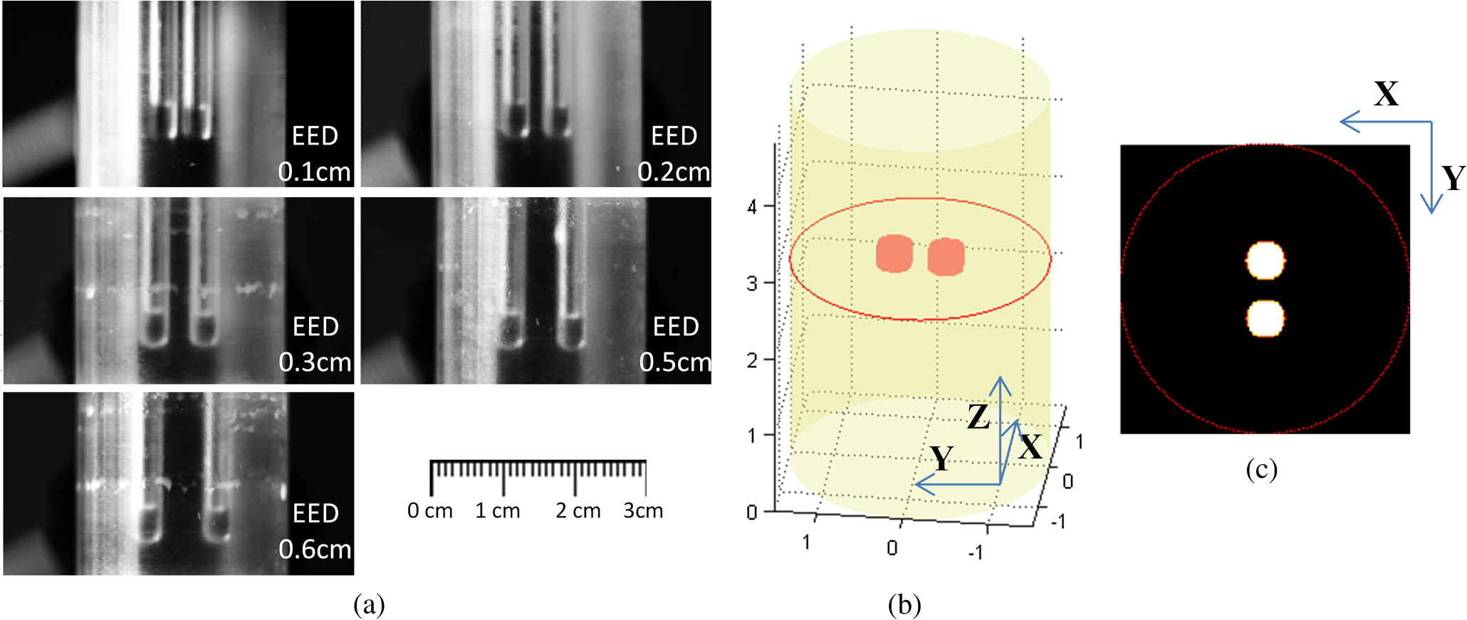

Figure 8 shows the fluorophore distribution reconstructed from the normalized Born average intensity using the Tikhonov, L1-Ls, and re-L1-NCG methods, respectively. All the images are normalized by the maximum of the reconstruction results and then displayed with the same color scale. The ﬂuorophore distribution is depicted using horizontal cross-sections at a height of 2.6 cm. In Fig. 8, the first two rows represent the reconstruction results obtained using the Tikhonov method. The third and fourth rows correspond to the cross-sections and 3-D renderings of the reconstruction results obtained using the L1-Ls method. The fifth and sixth rows correspond to the reconstruction results obtained using the re-L1-NCG algorithm. Five columns represent different EEDs, respectively.

Fig. 8

The reconstructed fluorescent targets of the physical phantom experiments. Five columns represent different EEDs. The reconstruction results are shown in the form of cross-section and 3-D rendering. (a1) to (e2) The reconstruction results obtained using the Tikhonov method. (f1) to (j2) The reconstruction results obtained using the L1-Ls method. (k1) to (o2) The reconstruction results obtained using the re-L1-NCG method.

When the EED is $< 0.3 cm$ , the two targets are barely distinguished using the Tikhonov method, as shown in Figs. 8(a2), 8(b2), and 8(c2). However, they can be clearly distinguished using the re-L1-NCG algorithm, as shown in Figs. 8(k2), 8(l2), and 8(m2). Compared with re-L1-NCG, Tikhonov as an L2-norm regularization method results in an oversmoothing effect (i.e., the volume of the reconstructed targets is much larger than the truth volume). In the simulation study with a cylinder model, high spatial resolution can be obtained using the L1-Ls algorithm. However, in the physical phantom, the reconstructed fluorescent targets obtained using the L1-Ls method cannot be well distinguished when the EED is $< 0.3 cm$ . By contrast, two fluorescent targets reconstructed using the re-L1-NCG algorithm can be distinguished when EED is 0.2 or 0.1 cm. In addition, the mean time consumed by L1-Ls was 364 s, while the mean time consumed by re-L1-NCG was only 34 s.

The profiles across the two targets at $x = 0$ (i.e., along the $y$ -axis direction) in the cross-sections of Fig. 8 are shown in Fig. 9 in order to better clarify the spatial resolution of the re-L1-NCG algorithm. As shown in Fig. 9, the peak locations of the profiles obtained with re-L1-NCG have a better match with the true locations, and the FWHM of the profiles obtained with Tikhonov is larger than that of L1-Ls and re-L1-NCG. The FWHM obtained using re-L1-NCG is reduced by 50 to 80% compared with the Tikhonov method. Figure 9 shows that, when using Tikhonov method, the contrast between the peak and valley values in the profiles is reduced as the EED decreases. It means that the spatial resolution obtained using Tikhonov is degraded with a decreased EED. However, when using re-L1-NCG algorithm, the contrast has slighter degradation when the EED is decreased. In Fig. 9(a), when the EED is decreased to 0.1 cm, the peaks corresponding to the two fluorescent targets can still be separated by using the re-L1-NCG algorithm. As shown in Figs. 9(c), 9(d), and 9(e), the L1-Ls method can obtain higher spatial resolution than the Tikhonov method. However, compared with the re-L1-NCG algorithm, the L1-Ls method obtains lower spatial resolution when the EED is small, which can be seen in Figs. 9(a), 9(b), and 9(c).

Fig. 9

Intensity profiles corresponding to different EEDs along the $y$ -axis direction in the cross-sections of Fig. 8.

To quantitatively analyze the spatial resolution, the performance metrics defined in Eq. (8) for each profile in Fig. 9 are listed in Table 2. As shown, higher spatial resolution (i.e., larger $R$ ) can be obtained using the re-L1-NCG algorithm.

Table 2

Quantification of spatial resolution calculated from Eq. (8) for the physical phantom study.

Edge-to-edge distance (cm)	0.1	0.2	0.3	0.5	0.6
$R$ (Tikhonov)	0.14	0.21	0.29	0.55	0.64
$R$ (restarted L1 regularization-based nonlinear conjugate gradient)	0.68	0.88	1	1	1
$R$ (L1-Ls)	0.77	0.65	0.95	0.99	1

4. Discussion and Conclusion

It is well known that the ill-posedness of FMT inverse problem causes relatively low spatial resolution in the reconstruction results. In this paper, enhanced spatial-resolution reconstruction is obtained using the re-L1-NCG algorithm, where the sparsity of the fluorophore distribution is used as a priori L1-norm penalty. As an L1 regularization-based algorithm, re-L1-NCG can preserve the high-frequency information like edges and reduce the noise of image effectively, when the fluorophore distribution is sparse. The re-L1-NCG algorithm is composed of inner and outer iterations. In view of the nondifferentiability of L1 penalty, L1-NCG was used in the inner iteration to solve the regularization optimization problem. Because the FMT inverse problem is severely ill-posed, the convergence speed of L1-NCG will deteriorate. However, L1-NCG can obtain an appropriate permission region without additional anatomical a priori information for the reconstructed fluorescent targets. Then the restarted strategy is adopted in the outer iteration to expedite the convergence of L1-NCG, by resetting the permission region and initial value. With the help of permission region, the computational speed can be increased with low memory consumption, which has been discussed in our previous work.²⁶ Thus, re-L1-NCG is an efficient algorithm for FMT reconstruction without anatomical a priori information for the reconstructed fluorescent targets. Moreover, the restarted strategy profits from the fact that the convergence of L1-NCG depends on the initial value. Thus, the proposed restarted strategy can be used for other algorithms benefiting from the initial value. In order to cancel out the position-dependent gain factors in the forward model, normalized Born approximation is adopted. By normalizing the columns of weight matrix $W$ , the high attenuation of emission light coming from deep fluorescence targets can be compensated.³⁷ For comparison, the Tikhonov (a representative L2-regularized method) and L1-Ls (a well-known L1-regularized method) are adopted.

The simulation and physical phantom studies demonstrate that the re-L1-NCG algorithm can significantly improve the spatial resolution of reconstruction results compared with the Tikhonov method, and re-L1-NCG has better performance than L1-Ls in terms of time consumption and spatial resolution, especially in the physical phantom study. The reconstruction results show that the re-L1-NCG algorithm has the ability to resolve targets with an EED of 0.1 cm, at a depth of 1.5 cm. The simulation study with digital mouse model demonstrates that the re-L1-NCG algorithm can obtain high contrast and spatial resolution when the FCR between fluorescent targets and background fluorescence is relatively large. For small FCR (i.e., $FCR = 10$ ), the fluorescent targets can still be reconstructed using re-L1-NCG, although the contrast between the reconstructed fluorescent targets and the background fluorescence is relatively low. In order to obtain high spatial resolution for small FCR, the transform sparsity of the fluorophore distribution can be included in the L1-regularized optimization function, which will be our future work.

For FMT reconstruction, the ill-posedness depends on several experimental parameters, including the scattering properties of the tissue, the position of the fluorescence targets in the tissue, the shape and size of the fluorescence targets, and the size of the discretization grid. It is difficult to compare the performance of different reconstruction algorithms because it depends on many factors, such as regularization parameters, number of iterations, and initial value. In this paper, the regularization parameters for the Tikhonov, L1-Ls, and re-L1-NCG methods were manually optimized through picking out suboptimal parameters in proper ranges. As the gradient projection approach, the L1-NCG method benefits from a good initial value. Thus, the warm-start technique can be adopted.⁴⁷ Automatic selection of the optimal or near-optimal regularization parameters by means of analyzing the ill-posedness will be our future work. In view of the advantage of total variation (TV) in preserving the boundary of large object and removing small features,⁴⁸ TV regularization will be incorporated in our future work.

For FMT reconstruction with high spatial resolution, another important factor lies in the accuracy of the photon propagation model itself.¹⁶^,⁴⁸ Except for the DE, the forward model based on RTE or higher-order approximations to RTE can be adopted to obtain higher spatial resolution solution, while the heterogeneous model can be utilized for more accurate solution. The re-L1-NCG algorithm can potentially be utilized in FMT reconstruction with these improved models, and in vivo small animal experiments will be conducted in the future.

Acknowledgments

This work is supported by the National Basic Research Program of China (973) under Grant No. 2011CB707701; the National Natural Science Foundation of China under Grant Nos. 81227901, 81271617, 61322101, 61361160418; the National Major Scientific Instrument and Equipment Development Project under Grant No. 2011YQ030114. Fei Liu is supported in part by the postdoctoral fellowship of Tsinghua-Peking Center for Life Sciences.

References

1.

V. Ntziachristoset al., “Looking and listening to light: the revolution of wholebody photonic imaging,” Nat. Biotechnol., 23 (3), 313 –320 (2005). http://dx.doi.org/10.1038/nbt1074 NABIF9 1087-0156 Google Scholar

2.

R. WeisslederV. Ntziachristos, “Shedding light onto live molecular targets,” Nat. Med., 9 (1), 123 –128 (2003). http://dx.doi.org/10.1038/nm0103-123 1078-8956 Google Scholar

3.

J. K. Willmannet al., “Molecular imaging in drug development,” Nat. Rev. Drug Discov., 7 (7), 591 –607 (2008). http://dx.doi.org/10.1038/nrd2290 NRDDAG 1474-1776 Google Scholar

4.

J. RaoA. Dragulescu-AndrasiH. Yao, “Fluorescence imaging in vivo: recent advances,” Curr. Opin. Biotechnol., 18 (1), 17 –25 (2007). http://dx.doi.org/10.1016/j.copbio.2007.01.003 CUOBE3 0958-1669 Google Scholar

5.

V. Ntziachristos, “Fluorescence molecular imaging,” Annu. Rev. Biomed. Eng., 8 1 –33 (2006). http://dx.doi.org/10.1146/annurev.bioeng.8.061505.095831 ARBEF7 1523-9829 Google Scholar

6.

J. MüllerA. WunderK. Licha, “Optical imaging,” Molecular Imaging in Oncology, 221 –246 Springer, Berlin, Heidelberg (2013). Google Scholar

7.

C. Gardneret al., “Improved in vivo fluorescence tomography and quantitation in small animals using a novel multiview, multispectral imaging system,” in Biomedical Optics and 3D Imaging, (2010). Google Scholar

8.

C. Liet al., “A three-dimensional multispectral fluorescence optical tomography imaging system for small animals based on a conical mirror design,” Opt. Express, 17 (9), 7571 (2009). http://dx.doi.org/10.1364/OE.17.007571 OPEXFF 1094-4087 Google Scholar

9.

A. J. Chaudhariet al., “Excitation spectroscopy in multispectral optical fluorescence tomography: methodology, feasibility and computer simulation studies,” Phys. Med. Biol., 54 (15), 4687 (2009). http://dx.doi.org/10.1088/0031-9155/54/15/004 PHMBA7 0031-9155 Google Scholar

10.

G. Zacharakiset al., “Volumetric tomography of fluorescent proteins through small animals in vivo,” Proc. Natl. Acad. Sci. U.S.A., 102 (51), 18252 –18257 (2005). http://dx.doi.org/10.1073/pnas.0504628102 PNASA6 0027-8424 Google Scholar

11.

J. Duttaet al., “Illumination pattern optimization for fluorescence tomography: theory and simulation studies,” Phys. Med. Biol., 55 (10), 2961 –2982 (2010). http://dx.doi.org/10.1088/0031-9155/55/10/011 PHMBA7 0031-9155 Google Scholar

12.

S. Bélangeret al., “Real-time diffuse optical tomography based on structured illumination,” J. Biomed. Opt., 15 (1), 016006 (2010). http://dx.doi.org/10.1117/1.3290818 JBOPFO 1083-3668 Google Scholar

13.

J. Duttaet al., “Optimal illumination patterns for fluorescence tomography,” in Proc. IEEE Intl. Symp. on Biomedical Imaging, 1275 –1278 (2009). Google Scholar

14.

A. JoshiW. BangerthE. M. Sevick-Muraca, “Non-contact fluorescence optical tomography with scanning patterned illumination,” Opt. Express, 14 (14), 6516 –6534 (2006). http://dx.doi.org/10.1364/OE.14.006516 OPEXFF 1094-4087 Google Scholar

15.

X. Caoet al., “Reconstruction for limited-projection fluorescence molecular tomography based on projected restarted conjugate gradient normal residual,” Opt. Lett., 36 (23), 4515 –4517 (2011). http://dx.doi.org/10.1364/OL.36.004515 OPLEDP 0146-9592 Google Scholar

16.

H. GaoH. Zhao, “Multilevel bioluminescence tomography based on radiative transfer equation. Part 1: L1 regularization,” Opt. Express, 18 (3), 1854 –1871 (2010). http://dx.doi.org/10.1364/OE.18.001854 OPEXFF 1094-4087 Google Scholar

17.

V. C. Kavuriet al., “Sparsity enhanced spatial resolution and depth localization in diffuse optical tomography,” Biomed. Opt. Express, 3 (5), 943 –957 (2012). http://dx.doi.org/10.1364/BOE.3.000943 BOEICL 2156-7085 Google Scholar

18.

P. Mohajeraniet al., “Optimal sparse solution for fluorescent diffuse optical tomography: theory and phantom experimental results,” Appl. Opt., 46 (10), 1679 –1685 (2007). http://dx.doi.org/10.1364/AO.46.001679 APOPAI 0003-6935 Google Scholar

19.

D. Hydeet al., “Data specific spatially varying regularization for multimodal fluorescence molecular tomography,” IEEE Trans. Med. Imaging, 29 (2), 365 –374 (2010). http://dx.doi.org/10.1109/TMI.2009.2031112 ITMID4 0278-0062 Google Scholar

20.

J. AxelssonJ. SvenssonS. Andersson-Engels, “Spatially varying regularization based on spectrally resolved fluorescence emission in fluorescence molecular tomography,” Opt. Express, 15 (21), 13574 –13584 (2007). http://dx.doi.org/10.1364/OE.15.013574 OPEXFF 1094-4087 Google Scholar

21.

B. Zhanget al., “Fluorescence tomography reconstruction with simultaneous positron emission tomography priors,” IEEE Trans. Multimedia, 15 (5), 1031 –1038 (2013). http://dx.doi.org/10.1109/TMM.2013.2244205 ITMUF8 1520-9210 Google Scholar

22.

J. Duttaet al., “Joint L1 and total variation regularization for fluorescence molecular tomography,” Phys. Med. Biol., 57 (6), 1459 –1476 (2012). http://dx.doi.org/10.1088/0031-9155/57/6/1459 PHMBA7 0031-9155 Google Scholar

23.

J. BaritauxK. HasslerM. Unser, “An efﬁcient numerical method for general Lp regularization in fluorescence molecular tomography,” IEEE Trans. Med. Imaging, 29 (4), 1075 –1087 (2010). http://dx.doi.org/10.1109/TMI.2010.2042814 ITMID4 0278-0062 Google Scholar

24.

D. Hanet al., “Efficient reconstruction method for L1 regularization in fluorescence molecular tomography,” Appl. Opt., 49 (36), 6930 –6937 (2010). http://dx.doi.org/10.1364/AO.49.006930 APOPAI 0003-6935 Google Scholar

25.

J. Shiet al., “Greedy reconstruction algorithm for fluorescence molecular tomography by means of truncated singular value decomposition conversion,” J. Opt. Soc. Am. A, 30 (3), 437 –447 (2013). http://dx.doi.org/10.1364/JOSAA.30.000437 JOAOD6 0740-3232 Google Scholar

26.

J. Shiet al., “Efficient L1 regularization-based reconstruction for fluorescent molecular tomography using restarted nonlinear conjugate gradient,” Opt. Lett., 38 (18), 3696 –3699 (2013). http://dx.doi.org/10.1364/OL.38.003696 OPLEDP 0146-9592 Google Scholar

27.

H. Puet al., “Separating structures of different fluorophore concentrations by principal component analysis on multispectral excitation-resolved fluorescence tomography images,” Biomed. Opt. Express, 4 (10), 1829 –1845 (2013). http://dx.doi.org/10.1364/BOE.4.001829 BOEICL 2156-7085 Google Scholar

28.

X. Liuet al., “Principal component analysis of dynamic fluorescence diffuse optical tomography images,” Opt. Express, 18 (6), 6300 –6314 (2010). http://dx.doi.org/10.1364/OE.18.006300 OPEXFF 1094-4087 Google Scholar

29.

B. Zhanget al., “Early-photon fluorescence tomography of a heterogeneous mouse model with the telegraph equation,” Appl. Opt., 50 (28), 5397 –5407 (2011). http://dx.doi.org/10.1364/AO.50.005397 APOPAI 0003-6935 Google Scholar

30.

V. Venugopalet al., “Full-field time-resolved fluorescence tomography of small animals,” Opt. Lett., 35 (19), 3189 –3191 (2010). http://dx.doi.org/10.1364/OL.35.003189 OPLEDP 0146-9592 Google Scholar

31.

M. LustigD. DonohoJ. M. Pauly, “Sparse MRI: the application of compressed sensing for rapid MR imaging,” Magn. Reson. Med., 58 (6), 1182 –1195 (2007). http://dx.doi.org/10.1002/(ISSN)1522-2594 MRMEEN 0740-3194 Google Scholar

32.

S. J. Kimet al., “An interior-point method for large-scale L1-regularized least squares,” IEEE J. Sel. Topics Signal Process., 1 (4), 606 –617 (2007). http://dx.doi.org/10.1109/JSTSP.2007.910971 1932-4553 Google Scholar

33.

S. R. Arridge, “Optical tomography in medical imaging,” Inverse Probl., 15 (2), 41 –93 (1999). http://dx.doi.org/10.1088/0266-5611/15/2/022 INPEEY 0266-5611 Google Scholar

34.

R. RoyA. GodavartyE. M. Sevick-Muraca, “Fluorescence-enhanced optical tomography using referenced measurements of heterogeneous media,” IEEE Trans. Med. Imaging, 22 (7), 824 –836 (2003). http://dx.doi.org/10.1109/TMI.2003.815072 ITMID4 0278-0062 Google Scholar

35.

A. SoubretJ. RipollV. Ntziachristos, “Accuracy of fluorescent tomography in the presence of heterogeneities: study of the normalized Born ratio,” IEEE Trans. Med. Imaging, 24 (10), 1377 –1386 (2005). http://dx.doi.org/10.1109/TMI.2005.857213 ITMID4 0278-0062 Google Scholar

36.

J. Ripollet al., “Fast analytical approximation for arbitrary geometries in diffuse optical tomography,” Opt. Lett., 27 (7), 527 –529 (2002). http://dx.doi.org/10.1364/OL.27.000527 OPLEDP 0146-9592 Google Scholar

37.

S. Ahnet al., “Fast iterative image reconstruction methods for fully 3D multispectral bioluminescence tomography,” Phys. Med. Biol., 53 (14), 3921 –3942 (2008). http://dx.doi.org/10.1088/0031-9155/53/14/013 PHMBA7 0031-9155 Google Scholar

38.

B. Wahlberget al., “An ADMM algorithm for a class of total variation regularized estimation problems,” (2014) http://www.stanford.edu/~boyd/papers/pdf/admm_tv_est.pdf March ). 2014). Google Scholar

39.

J. F. Abascalet al., “Fluorescence diffuse optical tomography using the split Bregman method,” Med. Phys., 38 (11), 6275 –6284 (2011). http://dx.doi.org/10.1118/1.3656063 MPHYA6 0094-2405 Google Scholar

40.

T. J. RudgeV. Y. SolovievS. R. Arridge, “Fast image reconstruction in fluoresence optical tomography using data compression,” Opt. Lett., 35 (5), 763 –765 (2010). http://dx.doi.org/10.1364/OL.35.000763 OPLEDP 0146-9592 Google Scholar

41.

T. LasserV. Ntziachristos, “Optimization of 360 projection fluorescence molecular tomography,” Med. Image Anal., 11 (4), 389 –399 (2007). http://dx.doi.org/10.1016/j.media.2007.04.003 MIAECY 1361-8415 Google Scholar

42.

V. Ntziachristoset al., “Fluorescence molecular tomography: new detection schemes for acquiring high information content measurements,” in IEEE Int. Symp. on Biomedical Imaging: From Nano to Macro, 1475 –1478 (2004). Google Scholar

43.

L. Zhanget al., “Three-dimensional scheme for time-domain ﬂuorescence molecular tomography based Laplace transforms with noise-robust factors,” Opt. Express, 16 (10), 7214 –7223 (2008). http://dx.doi.org/10.1364/OE.16.007214 OPEXFF 1094-4087 Google Scholar

44.

B. Dogdaset al., “Digimouse: a 3D whole body mouse atlas from CT and cryosection data,” Phys. Med. Biol., 52 (3), 577 –587 (2007). http://dx.doi.org/10.1088/0031-9155/52/3/003 PHMBA7 0031-9155 Google Scholar

45.

G. AlexandrakisF. R. RannouA. F. Chatziioannou, “Tomographic bioluminescence imaging by use of a combined optical-PET (OPET) system: a computer simulation feasibility study,” Phys. Med. Biol., 50 (17), 4225 –4241 (2005). http://dx.doi.org/10.1088/0031-9155/50/17/021 PHMBA7 0031-9155 Google Scholar

46.

F. Liuet al., “A parallel excitation based fluorescence molecular tomography system for whole-body simultaneous imaging of small animals,” Ann. Biomed. Eng., 38 (11), 3440 –3448 (2010). http://dx.doi.org/10.1007/s10439-010-0093-4 ABMECF 0090-6964 Google Scholar

47.

M. A. T. FigueiredoR. D. NowakS. J. Wright, “Gradient projection for sparse reconstruction: application to compressed sensing and other inverse problems,” IEEE J. Sel. Topics Signal Process., 1 (4), 586 –598 (2007). http://dx.doi.org/10.1109/JSTSP.2007.910281 1932-4553 Google Scholar

48.

H. GaoH. Zhao, “Multilevel bioluminescence tomography based on radiative transfer equation. Part 2: total variation and L1 data fidelity,” Opt. Express, 18 (3), 2894 –2912 (2010). http://dx.doi.org/10.1364/OE.18.002894 OPEXFF 1094-4087 Google Scholar

Biography

Junwei Shi received his MS degree from Xi’an Jiaotong University, Xi’an, Shaanxi, China, in 2011. Since 2011, he has been working toward the PhD degree in the Biomedical Engineering Department, Tsinghua University, Beijing, China. His research interest is fluorescence molecular tomography reconstruction algorithm.

Fei Liu received a BS degree in biomedical engineering from Zhejiang University, Zhejiang, China, in 2008. She is currently a PhD candidate in the Biomedical Engineering Department, Tsinghua University, Beijing, China. Her research interest is fluorescence molecular tomography for small animal imaging.

Gaunglei Zhang received the MS degree in biomedical engineering from Northwestern Polytechnical University, Xi’an, China, in 2007. He is currently a PhD candidate in the Biomedical Engineering Department, Tsinghua University, Beijing, China. His research interest is inverse problems of fluorescence molecular tomography.

Jianwen Luo received his BS and PhD degrees in biomedical engineering from Tsinghua University in 2000 and 2005, respectively. He was a postdoctoral research scientist from 2005 to 2009, and an associate research scientist from 2009 to 2011, in the Department of Biomedical Engineering at Columbia University. He became a professor at Tsinghua University in 2011, and was enrolled in the Thousand Young Talents Program in 2012. His research interest is biomedical imaging.

Jing Bai received the MS and PhD degrees from Drexel University in 1983 and 1985, respectively. From 1985 to 1987, she was a research associate and assistant professor at the Biomedical Engineering and Science Institute, Drexel University. In 1991, she became a professor in the Biomedical Engineering Department of Tsinghua University. Her current research interests include medical ultrasound and infrared imaging. She has authored or coauthored ten books and more than 300 journal papers.

Citation Download Citation

Junwei Shi, Fei Liu, Guanglei Zhang, Jianwen Luo, and Jing Bai "Enhanced spatial resolution in fluorescence molecular tomography using restarted L1-regularized nonlinear conjugate gradient algorithm," Journal of Biomedical Optics 19(4), 046018 (28 April 2014). https://doi.org/10.1117/1.JBO.19.4.046018

Published: 28 April 2014

Access the abstract

JOURNAL ARTICLE
13 PAGES

DOWNLOAD PAPER SAVE TO MY LIBRARY

GET CITATION

CITATIONS

Cited by 39 scholarly publications.

Explore citations on Lens.org

RIGHTS & PERMISSIONS

Get copyright permission Get copyright permission on Copyright Marketplace

KEYWORDS

Reconstruction algorithms

Spatial resolution

Luminescence

Detection and tracking algorithms

Fluorescence tomography

Tomography

Resolution enhancement technologies

1.

Introduction

2.

Method

2.1.

Model of Diffusion Equation

Eq. (1)

Eq. (2)

Eq. (3)

2.2.

FMT Reconstruction Based on L1 Regularization

Eq. (4)

Eq. (5)

Eq. (6)

Eq. (7)

Fig. 1

Eq. (8)

3.

Experiments and Results

3.1.

Simulation Studies: Cylinder Model

Fig. 2

Fig. 3

Table 1

3.2.

Simulation Studies: Digital Mouse Model

Fig. 4

Eq. (9)

Fig. 5

3.3.

Physical Phantom Study

Fig. 6

Fig. 7

Fig. 8

Fig. 9

Table 2

4.

Discussion and Conclusion

Acknowledgments

References

Biography

Show All Keywords

Keywords/Phrases

Search In:

Publication Years