1.

Introduction

Computerized methods of retinal imaging began in the 1970s. Initially there were difficulties with this technology being adopted by eye care professionals (ophthalmologists and optometrists).¹ With time, however, these difficulties were overcome through improvements in technology on one hand and a clearer evidence-based criteria for the diagnosis of retinal diseases on the other.¹ As a result, these tools are now available at a time when the incidence of retinal pathologies, such as diabetic retinopathy (DR) and age-related macular degeneration (AMD), is sharply increasing² and, in the case of DR, reaching pandemic proportions.² Computerized retinal imaging not only provides an enhanced analysis in clinical follow-up, but also screens for the presence of early stages of pathology. Furthermore, telemedicine allows such retinal images to be obtained from remote areas, thereby enabling diagnosis and treatment to occur when a specialized ocular expert is not present.³ Microaneurysms, hemorrhages, exudates and cotton wool spots, drusen, and abnormal and fragile new blood vessels are all indicators of retinal diseases. The tasks of image analysis in the case of DR involve, but is not limited to, early detection of red lesions (microaneurysms and hemorrhages) and subsequent development of bright lesions (exudates and cotton wool spots). In the case of AMD, the imaging needs to detect another bright lesion (drusen) forming in the macula.¹ Drusen are small yellow or white concretions that form in the retina and cause damage in the retinal layers directly underneath them. A high-resolution (HR) image contains more information and, hence, increases the accuracy in assessing the size and form and structure of a retinal lesion. Moreover, the ability to resolve micron scale retinal structures allows a better understanding of the biophysics and visual process.

The term resolution refers to the ability of an imaging instrument to reveal the fine details in an object. The resolution of an imaging device depends on the quality of its optics, recording (sensor) and display components, and the nature of the input source radiation. In this paper, the term resolution refers to the spatial resolution. Spatial resolution is further divided into axial and lateral resolution. Axial resolution is the ability to distinguish two closely spaced points in the direction parallel to the direction of the incident beam (Fig. 1). Medical techniques such as confocal microscopy, optical coherence tomography (OCT), and ultrasound provide images of an object in the axial direction. The axial resolution depends mostly upon the nature of the input source radiation. For example, the axial resolution of ultrasound is equal to half of the input spatial pulse length, whereas the axial resolution of OCT is equivalent to the coherence length of the incident light source. On the other hand, the lateral resolution is the ability of an instrument to distinguish two closely spaced points in the direction perpendicular to the direction of the incident beam (Fig. 1). The lateral resolution is determined by the width of the beam; the wider the beam, the poorer the lateral resolution. The lateral resolution of an imaging instrument depends mostly on its imaging optics.⁴ A high numerical aperture (NA) lens can be used to generate a small spot size that can improve the lateral resolution; however, the resolution achieved is rather limited. Furthermore, both monochromatic and chromatic aberration increases with increasing NA.⁵ Therefore, it is not beneficial to increase the NA beyond a certain limit. The spatial resolution of an imaging instrument can be improved by modifying the sensor in two ways. First, one can increase the pixel numbers, but at the cost of lower signal-to-noise ratio (SNR) and/or longer acquisition time.⁶ Second, the chip size can be increased; however, the chip size necessary to capture a very HR image would be very expensive.⁶ An interesting alternative to all these options is to use an image processing method called super-resolution (SR).⁷

Fig. 1

Illustration of axial and lateral resolution.

SR imaging was first introduced by Tsai and Huang⁸ in 1984. It is one of the most rapidly growing areas of research in image processing. A survey of different SR techniques can be found in Refs. 6 and 910. to 11. SR techniques are broadly divided into multiframe SR (classical approach) and single-frame SR. In multiframe SR technique, a set of low-resolution (LR) images acquired from the same scene is combined to reconstruct a single HR image. Multiple images can be taken using the same imaging instrument or different instruments. The goal is to obtain the missing information in one LR image from other LR images. This way the information contained in all LR images are fused to obtain an HR image.⁹ Several image fusion applications have been investigated in medical imaging.¹² In single-frame SR technique, the missing high-frequency information is added to the LR image using learning-based techniques. The learning-based techniques use HR training set images to learn the fine details and the learned information is used to estimate the missing details of the LR images.⁶

Retinal fundus is the interior of the eye that includes retina, macula, optic disc, and posterior pole. Fundus images are usually taken by a fundus camera and are used by eye care professionals for diagnosis and tracking of eye diseases. In fact, retina-related diagnosis is based largely on the fundus images. In this paper, we compare the performance of various frequently employed SR techniques and examine their suitability for the fundus retinal imaging. To the best of our knowledge, the SR techniques have not been fully applied to retinal images in the past. For each technique, peak SNR (PSNR) and the structural similarity (SSIM) between the super-resolved image and its original are computed. The PSNR is the peak SNR between the original and super-resolved image, in decibels. PSNR is calculated from the mean square error (MSE), which is the average error between the super-resolved image and its original. A higher value of PSNR indicates a better image quality. The SSIM index computes the similarity between the original and super-resolved image. The SSIM accounts the luminance, contrast, and structural changes between the two images. The rest of the paper is structured as follows. Section 2 describes the observation model for SR. The observation model relates the HR image with the observed LR images. Section 3 presents various multiframe SR techniques, where an HR image is obtained by combining a set of LR images. Section 4 presents the learning-based SR techniques. Comprehensive comparisons of various SR techniques using retinal images are included in Sec. 5. Finally, Sec. 6 provides the discussion and conclusion.

2.

Observation Model

It is important to know the parameters that degrade a retinal image before applying any SR method on it. Blur created either by defocus or motion degrades the retinal image quality. Sampling an object at a frequency less than the highest frequency contained in the object produces aliasing. Also, all retinal images contain some level of noise. These image degradation factors can be incorporated into a mathematical model that relates the HR image to the observed LR image. To be more precise, let $X$ be an original image, which is degraded by motion blur ($M$) followed by camera blur ($B$) and decimation effect ($D$). Furthermore, the image is deteriorated by the white Gaussian noise $\eta$ created during the acquisition process. The observation model that relates the HR image to the observed LR image is

The SR methods estimate the image degradation model $H$ and use it to reconstruct an HR image $X$ from a sequence of LR images $Y$. Figure 2 shows a schematic diagram of the observation model. By using different values of $k$ (i.e., different motion parameters, blur, decimation, and noise), different LR images can be created from an HR image. The practical values of $k$ for creating simulated LR images for this study are described in Sec. 5.

Fig. 2

Super-resolution observation model. The low-resolution (LR) images are the blurred, warped, decimated, and noisy version of a high-resolution (HR) image.

3.

Multiframe SR Approaches

In this technique, an HR image is reconstructed from a sequence of LR images. A schematic diagram is depicted in Fig. 3. There are a number of different approaches for reconstructing a single HR image by pooling information from multiple LR images. This paper includes only the most common reconstruction-based SR approaches.

Fig. 3

A framework of reconstruction-based super-resolution (SR) technique. An HR image can be reconstructed by pooling information from many LR images.

4.

Learning-Based SR Approaches

Learning-based SR methods extract the high-frequency information, which is lost during image acquisition process, from the external sources (training set images) and integrate this information with the input LR image to acquire a super-resolved image.^41–43 The schematic diagram of learning-based SR is depicted in Fig. 4. The training set consists of many HR images and their simulated LR versions. The performance of the learning-based SR methods highly depends upon the training set data. The training set images should have high-frequency information and be similar to the input LR image.⁴¹ To reduce the computational complexity, the learning-based methods are usually performed on the image patches. The learning-based SR methods include the following four stages as depicted in Fig. 5. First, the HR patches and their simulated LR version are stored in the training set in pairs. The features of the training set patches are extracted. A number of different types of feature extraction models can be used such as luminance values, DCT coefficients, wavelet coefficients, contourlet coefficients, PCA coefficients, gradient derivatives, Gaussian derivatives, Laplacian pyramid, steerable pyramid, feature extracted from bandpass filter, low- and high-pass frequency components, quaternion transformation, histogram of oriented gradients, etc. A summary of various feature extraction models is found in Ref. 41. Second, features of the input LR patches are extracted. Third, the features extracted from the input patches and training set patches are matched and the best matched pair from the training set is selected. In recent years, a number of learning methods have been proposed to match the features. The most common learning models are best matching, MRF, neighbor embedding, and sparse representation model.⁴¹ Fourth, the learned HR features are integrated into the input LR patch to achieve a super-resolved patch. Finally, all super-resolved patches are combined to generate the HR image.

Fig. 4

An illustration of learning-based SR.

Fig. 5

Flow chart of learning-based SR.

The example-based (EB) SR method proposed by Kim and Kwon⁴³ has outperformed several state-of-the-art algorithms in single-image SR. This method is based on the framework of Freeman et al.,⁴² which collects pairs of LR and HR image patches in the training stage. In the learning stage, each LR patch of the input image is compared to the stored training set LR patches, and using a nearest-neighbor search method a nearest LR patch and its corresponding HR pair are selected. However, this approach often results in a blurred image due to the inability of nearest neighbor. Kim and Kwon⁴³ modified this approach by replacing nearest-neighbor search with sparse kernel ridge regression. In their approach, kernel ridge regression is adopted to learn a map from input LR patch to training set’s HR and LR patch pairs. This method, however, also produces some blurring and ringing effects near the edges, which can be removed using postprocessing techniques.⁴³

Over the last century, there have been extensive studies on sparse representation algorithms. Sparse representation is the approximation of an image/signal with the linear combinations of only a small set of elementary signals called atoms. The atoms are chosen either from a predefined set of functions (analytical-based dictionary), such as DCT and wavelets, or learned from a training set (learning-based dictionary). The main advantage of these algorithms is that the signal representation coefficients are sparse, i.e., they have many zero coefficients and a few nonzero coefficients. To be more precise, consider a finite-dimensional discrete time signal $x\in R^N$ and an overcomplete dictionary $D\in R^{N\times K}$, $N<K$. The aim is to represent signal $x$ using dictionary $D$ such that the signal representation error ${\Vert D\alpha -x\Vert }_2$, where $\alpha$ is the sparse representation vector, is minimized. The sparse representation of a signal is obtained by solving the following optimization problem.⁴⁴

Sparse representation has become a major field of research in signal processing. Utilizing this approach, several researchers have proposed learning-based SR algorithms.^44–49 Sparse representation-based SR computes the sparse approximation of input LR patch and uses the coefficients of approximation to estimate an HR patch. In this method, two dictionaries $D_h$ and $D_l$ are jointly trained from HR and LR patches. There is a need to enforce the similarity of sparse coding between the LR ($j=D_l\beta$) and HR patch $l=D_h\alpha$. The dictionary extracted from the HR patch $D_h$ is applied with the sparse representation of the LR patch ($D_h\beta$) to recover the super-resolved patch. The schematic illustration of SR via sparse representation as proposed by Yang et al.⁴⁵ is shown in Fig. 6.

Fig. 6

Flow chart of SR via sparse representation algorithm.

In sparse representation-based approach, the final super-resolved image patch is generated from the combination of sparse coefficients of the LR patch and the HR dictionary; the performance of the method depends upon both the sparse coefficients of LR patch and the HR dictionary. Many researchers have proposed new algorithms to better estimate the HR dictionary and sparse coefficients of the LR image. Dong et al.⁴⁶ proposed a cluster-based sparse representation model called adaptive sparse domain selection (ASDS) to improve the dictionary. In this approach, the image patches are gathered into many clusters and a compact subdictionary is learned for each cluster. For each image patch, the best subdictionary can be selected that can reconstruct an image more accurately than a universal dictionary. Another study by Dong et al.⁴⁷ proposed sparse representation-based image interpolation through incorporating the image nonlocal self-similarities to the sparse representation model. The term self-similarity refers to the similarity of image pixel values or structure at different parts of the image. The algorithm included nonlocal autoregressive model as a new fidelity term to the sparse representation model, which reduces the coherence between the dictionaries and, consequently, makes sparse representation model more effective. Dong and colleagues not only estimated better HR dictionary for each image patch, but also utilized the image nonlocal self-similarity to obtain good estimation of the sparse representation coefficients of LR image. Recently, they have proposed two models for extracting sparse coding coefficients from the LR image as close to the original image as possible using nonlocal sparsity constraints. These are the centralized sparse representation (CSR) model⁴⁸ and the nonlocally CSR (NCSR) model.⁴⁹

5.

Simulations

MATLAB® software (version R2008a) was used to code and/or to run the programs. The MATLAB® codes were downloaded from the websites of respective authors, and the parameters of each method were set according to the values given in their corresponding papers. A computer with the operating system 64 bit version of Windows 7, Intel (R) Pentium (R) CPU G620T 2.2 GHz processor, and 4 GB RAM, was used to run the simulations. The screen resolution was $1920\times 1080$. Retinal fundus images taken with a fundus camera (Non-Mydriatic Auto Fundus Camera, Nidek AFC-230, Gamagōri, Aichi, Japan) were used to run the simulations. The images were taken from the right eye of one of the authors (D.T.) who has no ocular pathology. SR approaches were applied separately for real LR images and simulated LR images. Simulated LR images are viewed as the shifted, rotated, and downsampled version of an HR image. We cropped three important sections ($256\times 256\text{pixels}$) from three different fundus images to run SR in different parts of the fundus image. The cropped sections were the optic disc, macula, and retinal blood vessels, and are shown in Fig. 7. Four $128\times 128\text{pixels}$ LR images were created from these HR images. The shift and rotation parameters were adjusted manually. Horizontal and vertical displacements were set to (0,0), $(-3,2)$, (2,1), and $(-2,3)$) and rotation angles were set to (0, 5, 3, $-2$) deg, respectively, to create four LR images. The downsample factor was set to 2. Finally, Gaussian noise was added to the LR images to maintain a signal-to-noise ratio of 40 dB. The first LR image is the reference LR image, which is a downsampled version of the HR image, with the shift and rotation parameters zero. The reference LR images are shown in Fig. 7 with their original. Figure 8 shows all four LR images that were created from the cropped optic disc image. We used these simulated LR images to recover the original HR image (resolution $256\times 256$) using various SR methods.

Fig. 7

HR test images created by cropping three different sections of three different fundus images and their corresponding LR version.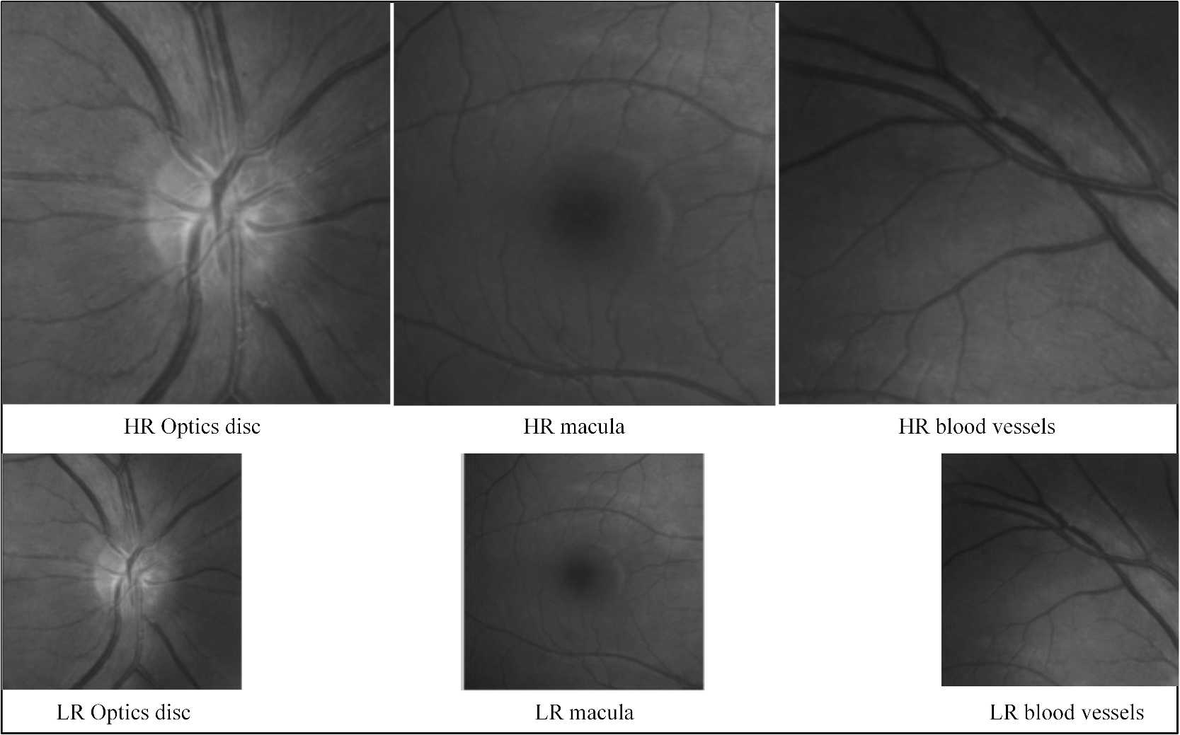

Fig. 8

LR images (resolution $128\times 128$) obtained from an optic disc using observation model. These images were used to run all the multiframe SR techniques.

Frequency domain SR approaches²⁴ were first examined on the simulated LR fundus images. These images were transformed into the Fourier domain, and shift and rotation parameters between the LR and reference images were calculated based on their low-frequency, aliasing part. Shifts were estimated from the central low-frequency components in which number of low-frequency components used were 10 and the rotations were estimated from a disc of radius 0.8. By incorporating these motion parameters on the simulated LR images, an HR image was reconstructed using cubic interpolation. Besides cubic interpolation, the performances of IBP,¹⁵ robust regularization,²⁹ and POCS²³ were also examined in Fourier domain. We employed MATLAB® software prepared by Vandewalle et al.²⁴ to implement these algorithms. For IBP, an upsampled version of the reference LR image was used as an initial estimate of HR image. The upsampling was performed using bicubic interpolation. The IBP created a set of LR images from the initial estimate of HR image using the motion parameters estimated in Fourier domain. The estimate was then updated by iteratively minimizing the error between the simulated LR images and test LR images based on the algorithm developed in Ref. 15. Robust regularization further incorporates a median estimator in the iterative process to achieve better results. We implemented the robust regularization algorithm proposed by Zomet and colleagues.²⁹ The POCS algorithm, which reconstructs an HR image using projection on convex sets, was examined only for the planar shift.

Similarly, Bayesian SR methods were studied, and their robustness on the LR fundus images was tested for various prior models. We used algorithms and MATLAB® software prepared by Villena et al.³³ for the simulation. TV,³¹ $l_1$ norm of the horizontal and vertical gradients,³² and SAR³³ were used as image prior models. The motion parameters and downsampled factor kept unchanged between the Fourier domain methods and Bayesian methods for fair comparison except for POCS in which planar rotation was not applied. The four simulated LR images were used as input. The algorithm utilized hierarchical Bayesian model where the model parameters, registration parameters, and HR image were estimated simultaneously from the LR images. Variational approximation was applied to estimate the posterior distributions of the unknowns. The algorithm terminated when either a maximum number of iterations ($k=100$) was reached or the criterion $[({\Vert x^k-x^{k-1}\Vert }^2)/({\Vert x^{k-1}\Vert }^2)]<{10}^{-4}$, where $x^k$ is the $k$’th estimated HR image, was satisfied. The Bayesian methods showed the highest PSNR value compared to the other multiframe SR methods. However, the TV norm, $l_1$ norm of the horizontal and vertical gradients, and SAR norm priors model led to oversmooth nonedge regions of the image. Figures 9, 10, and 11 show the results of various multiframe SR approaches applied to the LR images of optic disc, macula, and retinal blood vessels. Table 1 shows PSNR and SSIM indices between the original and the super-resolved images obtained from different multiframe SR approaches.

Fig. 9

Results from different multiframe SR approaches for LR optic disc images.

Fig. 10

Results from different multiframe SR approaches for LR macula images.

Fig. 11

Results from different multiframe SR approaches for LR blood vessels.

Single-image interpolation methods were also studied on retinal images. The input LR image was created by direct subsampling of the original image by a factor of 2. The LR retinal image was upscaled to its double size $256\times 256$ using nearest-neighbor, bilinear, and bicubic interpolations. The interpolated images were compared with the original image. The PSNR and SSIM indices for bicubic method were greater than those of the nearest-neighbor and bilinear interpolation. The complex interpolation methods, cubic spline,³⁰ NEDI (Ref. 20), and EGI (Ref. 21), were also applied to the downsampled LR images of optic disc, macula, and retinal blood vessels. Noise was not added to the LR image of single-image interpolation methods, so they showed better PSNR and SSIM indices. The comparisons between the various single-image interpolation approaches in terms of objective quality matrices (PSNR and SSIM) are shown in Table 2. A regularization-based SR with sparse maxing estimators (SME)³⁰ was also examined and showed better PSNR and SSIM indices.

Table 1

Peak signal-to-noise ratio (PSNR) and structural similarity (SSIM) indices between the original and the super-resolved images obtained from a set of low-resolution simulated images using different multiframe super-resolution (SR) approaches, best values in bold.

Table 2

PSNR and SSIM indices between the original and the reconstructed images obtained from various single-image SR approaches, best values in bold.

We examined the EB method proposed by Kim and Kwon⁴³ on the cropped fundus images. We chose this method since it has outperformed many state-of-the art algorithms and also because it removes blurring and ringing effects near the edges.⁴³ The input LR images were created by downsampling the original image by a factor of 2. Noise was not added to the downsampled image. The training set was created by randomly selecting HR generic images. The LR training images were obtained by blurring and subsampling HR images. Thus, the training set constituted a set of LR and HR image pairs. The algorithm was performed on image patches. In this method, the input LR patch was first interpolated by a factor of 2 using cubic interpolation. Next, kernel ridge regression was adopted to learn a map from input LR patch to training set image HR and LR patch pairs. The regression provided a set of candidate images. The super-resolved image was obtained by combing through candidate images based on estimated confidences. The artifacts around the edges of the reconstructed image were removed by utilizing image prior regularization term. Better PSNR and SSIM values are noticed in this method.

Similarly, sparse representation-based SR techniques were examined on the LR fundus image. We extracted $5\times 5$ patches with overlap of 1 pixel between adjacent patches from the input image. The HR dictionaries and sparse coefficients were learned from both the training set HR images and LR test image. We used the method and software proposed by Yang et al.⁴⁴ to run the simulation. In addition, ASDS,⁴⁶ sparse interpolation,⁴⁷ CSR,⁴⁸ and the most recent NCSR (Ref. 49) methods proposed by Dong et al. were also implemented on LR patches. The latter two methods introduced the centralized sparsity constraint by exploiting nonlocal statics. Both the local sparsity and nonlocal sparsity constraints are combined in this approach. The centralized sparse representation approach approximates the sparse coefficients of the LR image as closely as the original HR image does, which results in better image reconstruction and, hence, better PSNR and SSIM indices. Figures 12, 13, and 14 show the results of various single-image SR approaches applied to the LR images of optic disc, macula, and retinal blood vessels.

Fig. 12

Results from various single-image SR approaches for LR optic disc images.

Fig. 13

Results from various single-image SR approaches for LR macula images.

Fig. 14

Results from various single-image SR approaches for LR blood vessel images.

Finally, multiframe SR techniques were examined on the multiple real retinal images. A fundus camera was fixed manually on the right eye of one of the authors (D.T.) and six consecutive images were taken. The participant’s head was fixed using chin rest. To eliminate pupil constriction, one drop of pupil dilating agent (Tropicamide 1%) was used in the eye. The accommodation effects were also minimized by the dilating agent by paralyzing the ciliary muscles. Six images were acquired with small shifts and rotations due to the eye motions. The images were then cropped to obtain the desired sections. We cropped a small retinal blood vessel section of the fundus image in this study. The sizes of the cropped sections were $128\times 128\text{pixels}$. One such section is shown in Fig. 15 (top left corner).

Fig. 15

Results from various multiframe SR approaches for real retinal images.

In the Fourier domain, the shifts between the images were estimated from the central 5% of the frequency and the rotations were estimated from a disc of radius 0.6 as described by Vandewalle et al.²⁴ The images were registered in the Fourier domain and then reconstructed to obtain an HR image using cubic interpolation. The resolution was increased by a factor of two. The robust regularization, IBP, and POCS were also tested on the real images. The results showed that cubic interpolation and POCS methods estimated the blur HR images. These images are worse than the image estimated by a single-image bicubic interpolation method, while the HR images estimated by IBP and robust regularization have better visual quality.

A hierarchical Bayesian algorithm was used to estimate the registration parameters in Bayesian methods and the blur was assumed to be a $3\times 3$ Gaussian with variance 1. We examined TV-prior, L1-prior, and SAR-prior models, but these models led to oversmooth nonedge regions of the image; therefore, combined TV-SAR and L1-SAR prior models were used as described by Villena et al.³³ The HR images obtained from these methods are shown in Fig. 15. The image obtained from single-image bicubic interpolation is also shown for comparison. The HR images suffered from registration errors likely due to the fact that most of the SR algorithms work only with planar motion and rotations. The real images, especially retinal images taken from a fundus camera, may have nonplanar motions due to the eye motion. A more precise knowledge of motion parameters is needed to solve this problem. The registration error may also be minimized by taking images from dynamic instruments. Last but not least, we examined blind deconvolution-based SR approach to combine multiple LR images to estimate an HR image as described by Sroubek and Flusser.⁴⁰ This method does not assume any prior information about the blur; it requires only the approximate size of the blur. In our case, we set $3\times 3$ blur kernel size. The algorithm built and minimized a regularized energy function given in Eq. (5) with respect to original image and blur. The regularization is conducted in both the image and blur domain. TV regularization was used for our simulation. The HR image predicted by a blind deconvolution method showed a more even spread of the brightness and the edges are sharper and clearer. Among all the above multiframe SR techniques, blind deconvolution showed best results for our LR images.

6.

Discussion and Conclusion

In this paper, we demonstrated the possibility of resolution enhancement of retinal images using SR techniques. Three important sections of the fundus images were considered for the simulations: optic disc, macula, and retinal blood vessels. In the first part, we simulated four LR images by shifting, rotating, downsampling, and adding Gaussian noise to an HR image. A number of important features of the fundus image are missing or less clearly visible in the LR images. For example, the arteries and veins emerging from the margins of the optic disc are less clearly visible. The connections between the optic disc and some of the blood vessels are not distinct in the LR optic disc images. The borderlines of blood vessels are less distinct in retinal blood vessels image. Similarly, there are several tiny arteries (cilioretinal arteries) supplying additional blood to the macular region that are also less clearly visible in LR macula images. In addition, the background of the retina is unclear, so recognition of the cilioretinal arteries is also difficult. The foveal reflex is considerably dim in LR macula images. The images were taken from a healthy normal eye; the difference might be more distinct in pathological eyes.

SR techniques give magnified image by fusing multiple LR images. The features of an image are also magnified in the same factor, so they are visually clearer in a larger image. This can be seen in many super-resolved images shown in Figs. 9 to 14. The features that are visually less distinct in LR images are more distinct in super-resolved image and the connection between the optic disc and blood vessels is comparatively clearer in super-resolved images given by SME, EB (Ref. 43), and sparse representation⁴⁴ methods (Fig. 12). However, some SR techniques, for example, sparse interpolation and ASDS, oversmoothed the image, so the important features are lost from the image. The cilioretinal arteries and foveal reflex in super-resolved images given by EB,⁴³ SME, and sparse⁴⁴ methods are as clear as in the original image, while they are significantly smoothed in super-resolved image obtained from sparse interpolation and ASDS methods (Fig. 13). The other SR techniques show intermediate performance. The super-resolved images have recovered many image features; however, lost edges or textures during the decimation process cannot be recovered completely. The EB (Ref. 43) and sparse representation⁴⁴ methods show good results and can be used when sufficient number of input LR images are unavailable and/or when higher resolution factor is required. The performance of these algorithms may be improved by using a larger set of training images and by using more relevant learning method.

In the second part, we implemented SR techniques on cropped version of six multiple acquisition retinal images taken with a fundus camera. The real images were first normalized, which reduced the effect of different levels of illumination in different images. The Fourier method²⁴ was used to estimate the registration parameters and then these parameters were used to fuse LR images. The Fourier-based cubic interpolation method significantly blurred the reconstructed image. The IBP, robust regularization, and single-image bicubic interpolation method introduced small amount of ringing effect; however, they preserved most of the image features. The Bayesian approaches performed a joint registration and fusion tasks together. They provided visually pleasant image; however, the HR image reconstructed by the Bayesian approaches were oversmoothed and many image details were lost. The blind deconvolution provided much sharper and cleaner reconstructed image than others; however, the HR image was not free of artifacts. Nevertheless, the algorithm is more realistic because it does not need prior information of the blur. In the real image SR approaches, we utilized only six LR images to perform SR; better results can be obtained if number of LR image is increased. Meitav and Ribak⁵⁰ used $>200$ retinal LR images to achieve an HR image using a weighted average method. Furthermore, the registration methods are restricted to the planar translational and rotational; however, the eye movements may induce nonplanar variations between LR images. The variations in the ocular surface, such as dynamic nature of the tear film, accommodation and cardiopulmonary effect of the eye, may result in different levels and types of variations between the LR retinal images. Small subpixel error in the registration may result in different estimation. Therefore, robust motion estimation algorithm is essential to perform SR in retinal images. Furthermore, many algorithms, including Bayesian approaches, assume spatially uniform Gaussian blur, which is usually impractical. To avoid damage to the eye, the retinal images are taken in the low-light condition, and therefore, they suffer from low SNR. Most of the SR algorithms deteriorate when noise is present in the image; therefore, a method that is more robust to noise but can also preserve image features is essential.

In summary, we demonstrated resolution enhancement of retinal images using image processing methods. While we investigated the performance of various SR techniques, we are unable to present the details of each method. The reader is advised to consult the related reference papers for specific implementation details. Since the codes were downloaded from the websites of respective authors and the parameters of each method were set according to the values given in their corresponding papers, the differences in PSNRs and SSIMs between various SR approaches may be due to the differences in techniques, and/or their parameters. We refer the interested readers to visit the webpage ∼ http://quark.uwaterloo.ca/~dthapa, which contains the MATLAB® source code for various SR techniques developed by several groups of researchers.