Optoacoustic characterization of prostate cancer in an in vivo transgenic murine model

Michelle P. Patterson; Christopher B. Riley; Michael C. Kolios; William M. Whelan

doi:10.1117/1.JBO.19.5.056008

9 May 2014 Optoacoustic characterization of prostate cancer in an in vivo transgenic murine model

Michelle P. Patterson, Christopher B. Riley, Michael C. Kolios, William M. Whelan

Author Affiliations +

Journal of Biomedical Optics, Vol. 19, Issue 5, 056008 (May 2014). https://doi.org/10.1117/1.JBO.19.5.056008

Abstract

Optoacoustic (OA) imaging was employed to distinguish normal from neoplastic tissues in a transgenic murine model of prostate cancer. OA images of five tumor-bearing mice and five age-matched controls across a 14 mm×14 mm region of interest (ROI) on the lower abdomen were acquired using a reverse-mode OA imaging system (Seno Medical Instruments Inc., San Antonio, Texas). Neoplastic prostate tissue was identified based on the OA signal amplitude in combination with spectral analysis of the OA radio frequency (RF) data. Integration of the signal amplitude images was performed to construct two-dimensional images of the ROI. The prostate tumors generated higher amplitude signals than those of the surrounding tissues, with contrast ratios ranging from 31 to 36 dB. The RF spectrum analysis showed significant differences between the tumor and the control mice. The midband fit was higher by 5 dB (62%), the intercept higher by 4 dB (57%) and the spectral slope higher by 0.4 dB/MHz (50%) for neoplastic prostate tissue compared to normal tissues in the control mice. The results demonstrate that OA offers high contrast imaging of prostate cancer in vivo.

1. Introduction

Conventional imaging techniques for prostate cancer, such as ultrasound, computed tomography, and magnetic resonance imaging, are used to identify abnormal areas in the prostate that are then biopsied for a definitive diagnosis. These imaging techniques do not reliably distinguish neoplastic from healthy prostate tissue,¹ leading to the large sampling error associated with biopsies. A sensitivity of only 50% is estimated for these techniques.² The ability to accurately visualize neoplastic regions in the prostate would improve biopsy targeting.

One of the most common techniques used for local grading of the prostate is transrectal ultrasound (TRUS) because it can be performed in real time. TRUS systems that utilize transducers in the 5 to 7 MHz range³ can provide an acceptable resolution of 0.3 to 0.5 mm.⁴ However, the accuracy of this technique is reported to be less than 50% to 60% with respect to the detection of prostate cancer, due largely to the weak contrast at depth in soft tissues.⁵^–⁷ Conventional diagnosis is currently based solely on the detection of gross anatomic properties of tissues. Recent techniques have been developed that probe tissue microstructure based on the spectral analysis of radio frequency (RF) data;⁸^,⁹ however, these ultrasonic techniques do not provide any information on the oxygen saturation or hemoglobin concentration of the tissue, both of which are often altered with neoplasia.¹⁰^,¹¹ Pure optical imaging techniques, such as diffuse optical tomography (DOT), are being investigated as possible targeting technologies for prostate cancer because of their ability to achieve adequate contrast in soft tissues¹²^,¹³ and their ability to measure the oxygen saturation and hemoglobin concentrations of the tissues. These techniques, however, suffer from strong light scattering in biological tissues,¹² resulting in either very limited imaging depth ( $< 1 mm$ ), as in optical coherence tomography, or limited resolution, as in DOT.¹⁰

Optoacoustic (OA) imaging overcomes the limitations described by merging the contrast capability of optical imaging with the resolution of ultrasound imaging.¹³ The quality of contrast in OA imaging is related to the optical properties, as in pure optical imaging, and the thermomechanical properties of the target while the resolution and the maximum imaging depth are scalable with the ultrasonic frequency, as in ultrasound imaging.¹⁰ Consequently, OA imaging can provide high contrast images with good resolution and penetration depth in soft tissue.¹⁴^,¹⁵

This emerging technique of OA exposes tissues to nanosecond pulsed laser light, which induces tissue-generated acoustic waves that are detected using wide band transducers.¹⁴^,¹⁵ The amplitude of an OA signal is largely dependent upon the optical absorption properties of the target tissues. Solid tumours often have increased blood flow, and therefore hemoglobin concentration, compared to healthy tissue.¹⁶^,¹⁷ The OA approach takes advantage of the high optical absorption of hemoglobin compared with other tissue components at wavelengths in the visible and near-infrared range to generate higher amplitude signals in regions with higher hemoglobin concentrations.¹⁴^,¹⁵ High resolution images of the mouse vasculature have been published by a number of groups.¹⁸^–²² The frequency content of the generated OA sound waves is broadband, and the detected signals are limited by the finite bandwidth of the ultrasound imaging transducers and the frequency dependent attenuation of ultrasound in tissues.²³ The frequency content of the OA RF signals may reflect the anatomical properties of the absorbing structures in a manner similar to the established techniques involving spectral analysis of ultrasound RF data.⁹^,²⁴^,²⁵ Theoretical work has shown that frequency characteristics of OA signals can differentiate between normal and neoplastic tissues even when it is not possible to resolve individual blood vessels;²⁵ an important consideration, since many OA imaging systems cannot resolve individual blood vessels at the depth of the prostate in humans [up to 10 cm (Ref. 26)].²⁷^,²⁸

Spectrum analysis of ultrasound RF data and its relation to tissue microstructure has been well described.²⁹ The size of the scattering structures compared to the wavelength of the incident ultrasound modifies the frequency content of the backscattered signal.³⁰ Therefore, the frequency analysis of the ultrasound backscatter RF signals holds useful information about the medium subresolution structures. Large databases have been developed, which are used with statistical classifiers to identify specific tissue types from spectral image data.⁸ Analysis of the frequency components of the RF signals improves the diagnostic capabilities of conventional ultrasound imaging.⁸^,²⁹^,³¹

RF data are collected in OA imaging wherein the size of the absorbing structure contributes to the frequency content of the OA signal.³² Spectrum analysis of RF OA signals generated by blood vessel phantoms (cylindrical tubes filled with ink and embedded into gelatin) shows a relationship between the spectral components and the diameter of the cylinders.³³ Spectrum analysis of high-frequency OA signals from ex vivo ocular tissue has also shown changes in the midband fit and slope around the pigmented iris.³⁴ Thus, the relationship between the spectral components of OA data is likely linked to the physical properties of the target and, more specifically, the spatial distribution of the hemoglobin concentration within the tissues. Hence, quantitative measurements may allow for databases to be established for OAs, which, along with statistical classifiers, may be used to identify tissue types from amplitude images and RF analysis.²⁵ It may also offer additional information on the target physiology and vascular morphology.

In this work, we utilized a low resolution, high contrast reverse-mode OA imaging system. OA amplitude and frequency data were obtained from transgenic mice that develop prostate adenocarcinoma and age-matched controls. We posit that the analysis of the OA frequency components arising from nonresolvable tissue structures can be used to distinguish normal from neoplastic tissues.

2. Materials and Methods

2.1.

Animal Model

The transgenic adenocarcinoma of the mouse prostate (TRAMP) model develops tumors similar to those reported in the human clinical prostate disease.³⁵^,³⁶ TRAMP mice develop spontaneous autochthonous prostate cancer with distant site metastasis.³⁶ The tumor development begins as androgen-dependent growth and then progresses to androgen-independent growth, a progression similar to that of the human disease.³⁷ The tumors originate and develop within the prostate gland, which means they cannot be palpated or visualized in the animal prior to imaging (unless evaluated in their late stages), unlike many other implanted tumor models. At the tissue level, the TRAMP model also displays prostatic intraepithelial neoplasia prior to tumor formation.³⁵

TRAMP mice form prostate tumors as early as 12 weeks of age, with metastasis as early as 24 weeks of age.³⁸ In this study, we used five TRAMP mice and five age-matched controls [C57BL/6J (wild type)] (Jackson Laboratories Inc., Bar Harbor, Maine).

2.2.

OA Image Acquisition

All procedures performed in this study were approved by the Animal Care Committee of the University of Prince Edward Island in accordance with the guidelines of the Canadian Council for Animal Care. Imaging took place between 24 and 28 weeks of age. Prior to imaging, each animal was placed in an anesthetic induction chamber and anesthetized with 2.5% isoflurane in 100% oxygen. Once anesthetized, the hair on the lower abdomen of the animal was removed using a chemical hair remover (Nair®, Church & Dwight Corporation Inc., Ontario, Canada) and the area to be imaged was marked using a permanent marker. The animal was maintained under general anesthesia (2.5% isoflurane in 100% oxygen), secured to a vertical holder, and lowered up to the neck in a water bath that contained the laser fibers and transducer. Imaging in water is required to optimize acoustic coupling.

The imaging system (Seno Medical Instruments Inc., San Antonio, Texas) consists of a Nd:YAG pumped Ti:Sapphire laser operating at 775 nm and an eight-element piezo-electric annular transducer array (Fig. 1). The array offers dynamic focusing capabilities, which allows for structures lying on the array axis to be localized along a large depth of field.³⁹

Fig. 1

The small animal OA imaging system. Laser optical path intercepts at 25 mm from the transducer that is located beneath a camera used for image positioning. The animal (target) remained stationary as optoacoustic (OA) signals were acquired by a raster scan of a $14 mm \times 14 mm$ region of the lower abdomen.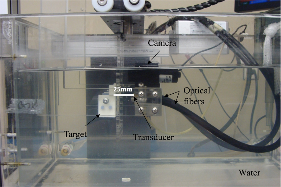

The transducer array has a central frequency of 5 MHz with a $- 6 dB$ bandwidth of 60%, a focal point at 25 mm, a focal length of 10 mm, and a focal width of 0.5 mm. The bifurcated optical fiber bundle delivered 6 ns pulses at a 10 Hz repetition rate and 20 mJ of energy per pulse. This is below the maximum permissible exposure limit of $100 mJ / {cm}^{2}$ at 775 nm as per the American National Standards Institute.⁴⁰ Throughout the imaging process, the mouse was held stationary as the fiber bundles and transducer array performed a raster scan across the selected area, moving in 0.2 mm steps and acquiring 4 OA signals at each position for averaging. The OA data were acquired from a $14 \times 14 mm$ region of interest (ROI_scan) at the lower abdomen of the mice that included the prostate region. The ROI_scan was defined by a marked outline drawn on the mouse. The total imaging time was approximately 1.4 h. This imaging time is a result of the raster approach, which, for our system, requires 1 s acquisition time at each step (including averaging), and there are approximately 4900 steps for each image.

Immediately following the image acquisition, each mouse was euthanized with an intracardiac injection of sodium pentobarbital ( $65 mg / kg$ ). Three TRAMP and age-matched control mice pairs were flash frozen in liquid nitrogen, in an upright position on the holder at all times to reduce organ migration. The lower abdomen was dissected and 100 μm lateral cryosections were acquired for gross anatomical comparison with the OA images using a cryostat. The other two TRAMP and age-matched control pairs were immediately dissected following euthanasia. The prostate, seminal vesicles, and any suspected abnormal tissues were fixed in a standard biological nitrogen fixation solution for histological processing. The tissue was sectioned and examined for evidence of prostate adenocarcinoma. The ROI_scan that was marked using a permanent marker prior to imaging was used to align the OA images with the cryosection photographs and histological sections.

2.3.

Signal Amplitude Analysis

For the signal amplitude analysis, OA data from a 3 μs time window were extracted from each RF line. This time window corresponded to a 5-mm depth, beginning 1 mm beneath the front surface of the animal (and at the same depth in the age-matched control). This removed the typically strong signals acquired from the animal skin surface and included data from tissue regions that included the prostate. The Hilbert transform was applied to all RF data.²⁷^,⁴¹ The signal strength is presented as arbitrary units, and all data were collected with the same constant gain settings.

In order to account for optical attenuation by tissues that reduces the light available at depth for OA wave generation, we have employed a depth-dependent signal correction to each A-line. This is somewhat analogous to the use of time gain controls in ultrasound imaging to account for acoustic attenuation. However, optical attenuation is significantly greater than the acoustic attenuation below 10 MHz in tissues.²⁷

The large aperture fiber bundles produce uncollimated light beams incident on the tissue surface. Hence, the subsurface fluence $I (z)$ at depth $z$ is diffuse and, as such, can be described using the effective attenuation coefficient, $μ_{eff}$ , according to Cox et al.⁴²

Eq. (1)

I (z) = I_{o} e^{- μ_{eff} z} .

An effective attenuation coefficient of $3.1 {cm}^{- 1}$ was used as reported for rat prostate tumors.⁴³ The final form of the correction factor was

Eq. (2)

{OA}_{corr} (z) = {OA}_{HT} (z) e^{μ_{eff} z} .

A MATLAB® (The MathWorks Inc., Natick, Massachusetts) based script was developed and used to apply the attenuation estimate to the signals. Such a correction is important given the variation in tumor depths that can occur among the TRAMP mice cohort.

The signal within each 3 μs time window was integrated and projected onto a two-dimensional (2-D) plane to form an image. A $2 mm \times 2 mm$ ROI was used for analysis (ROI_analysis). This region size was chosen so that the ROI_analysis, if placed in the center of the smallest tumor, would be on-tumor tissue despite an estimated alignment uncertainty of 2 mm between the OA images and the cryosections/histological images. This alignment uncertainty includes a 0.5 mm measured uncertainty in the camera positioning, and a 1.5 mm estimated uncertainty due to potential organ migration during image acquisition and prior to freezing.

Contrast values were determined between the on-tumor and adjacent (off-tumor) tissues within the OA image of the TRAMP mice, as well as between the tumor and the normal prostate region of the age-matched control. Contrast was measured by subtracting the average signal value within the ROI_analysis on control tissue from the average signal value within the ROI_analysis on tumor tissue and dividing by the standard deviation.⁴⁴^,⁴⁵

The tumor boundary was determined using the full width half maximum (FWHM) of the signal in the 2-D image. Hence, regions with signals greater than half the maximum signal were defined as “on-tumor.”²²

2.4.

RF Spectrum Analysis

A spectrum analysis technique commonly performed on ultrasonic backscatter RF data was used for this analysis.²⁹ To obtain the sensitivity of the transducer at different frequencies, a calibrated power spectrum was obtained by using a 200-nm thick gold film. The film was deposited onto a thin microscope cover slide with no annealing. The gold film was used because it has a broad OA power spectrum as well as a flat response in the known bandwidth of the transducer thus providing a good measure of the transducer response.⁴⁶ OA measurements were obtained across an area of approximately $1 {cm}^{2}$ at 775 nm illumination. A total of 20 OA signals were recorded. This is referred to as the calibrated power spectrum.

The fast Fourier transform was applied to the tissue RF data to calculate the RF echo spectrum. The mean of the squared spectral magnitudes is the averaged power spectrum (APS). The APS was converted into the decibel (dB) scale. A calibrated power spectrum is subtracted from the converted APS to remove any system-specific artifacts caused by the transducer characteristics at the focus and system electronics.

Values were calculated over a 5-mm depth beginning 1 mm before at the front surface of the tumor. The same $2 {mm}^{2}$ ROI_analysis used for the contrast measurements was used. Values were calculated at each position (i.e., every 0.2 mm) within the $2 {mm}^{2}$ ROI_analysis and were averaged. The same acquisition plane was used on the TRAMP mice and age-matched controls.

A sliding Hamming window was employed that has been shown to significantly reduce noise in the spectrum analysis of ultrasound data.²⁹ The Hamming window had a width of 1 mm and moved in 0.5 mm steps along the axial direction. A 1 mm window was chosen so that approximately three acoustic wavelengths (at the central frequency of the transducer) were contained in each window. The power spectrum at each location was the average of the measured spectrum in each Hamming window.

A linear regression was performed on the APS between 1 and 6 MHz and the midband fit, slope, and intercept extracted from the fit. This region was chosen based on the approximate linearity of the dataset and the high signal-to-noise ratio (SNR of 5.3 dB) within these frequencies. The statistical spread of these parameters for ultrasound RF data has been previously established by others.²⁹ A paired $t$ -test was used to compare the spectral parameters between normal and neoplastic tissue.

3. Results

3.1.

OA Imaging

Representative TRAMP and age-matched control cryosection and integrated OA signal amplitude images are shown in Fig. 2. Approximate areas imaged on the animals are represented by black outlines. The cryosection images of both sets of control and TRAMP mice were taken from the same depth beneath the surface of the animal, 6.0 and 7.9 mm, respectively, which corresponds to the maximum coronal tumor dimension in the TRAMP mice (determined from the cryosections). Each TRAMP image was normalized to its maximum signal value, and each control image was normalized to the maximum signal value from the image of its age-matched TRAMP. The OA image of the TRAMP mouse in Fig. 2(b) shows an increase in signal amplitude in the region of the tumor and relatively sharp decreases in the signal at the border of the tumor. The signals obtained from the control mouse are typically $< 0.5$ a.u. and therefore beneath our defined threshold of tumor tissue (defined in Sec. 2 using the FWHM and therefore above 0.5 a.u.). The tumor of the second TRAMP mouse was less vascularized compared to that of the first TRAMP mouse and has therefore been outlined in Fig. 2(e) for easier visualization. Again the tumor is visible in the corresponding OA image, Fig. 2(f), and the OA predicted vertical and horizontal dimensions are 7.0 and 6.0 mm, which reasonably agree with actual dimensions.

Fig. 2

Coronal cryosection images of TRAMP tumor-bearing mice (a and e) with maximum tumor diameters of 9.0 and 7.0 mm, and age-matched control mice (c and g). Approximate areas imaged on animals are represented by black outlines. Corresponding coronal integrated signal amplitude images of tumor-bearing TRAMP mice (b and f) with OA predicted tumor diameters of 8.8 and 7.0 mm, respectively and age-matched control mice (d and h). Both sets of OA images (TRAMP and age-matched control) were normalized to the maximum signal value of the TRAMP image. The tumor in the second TRAMP mouse (e) is much less vascularized than that of the first TRAMP mouse (a) and has been outlined for easier visualization.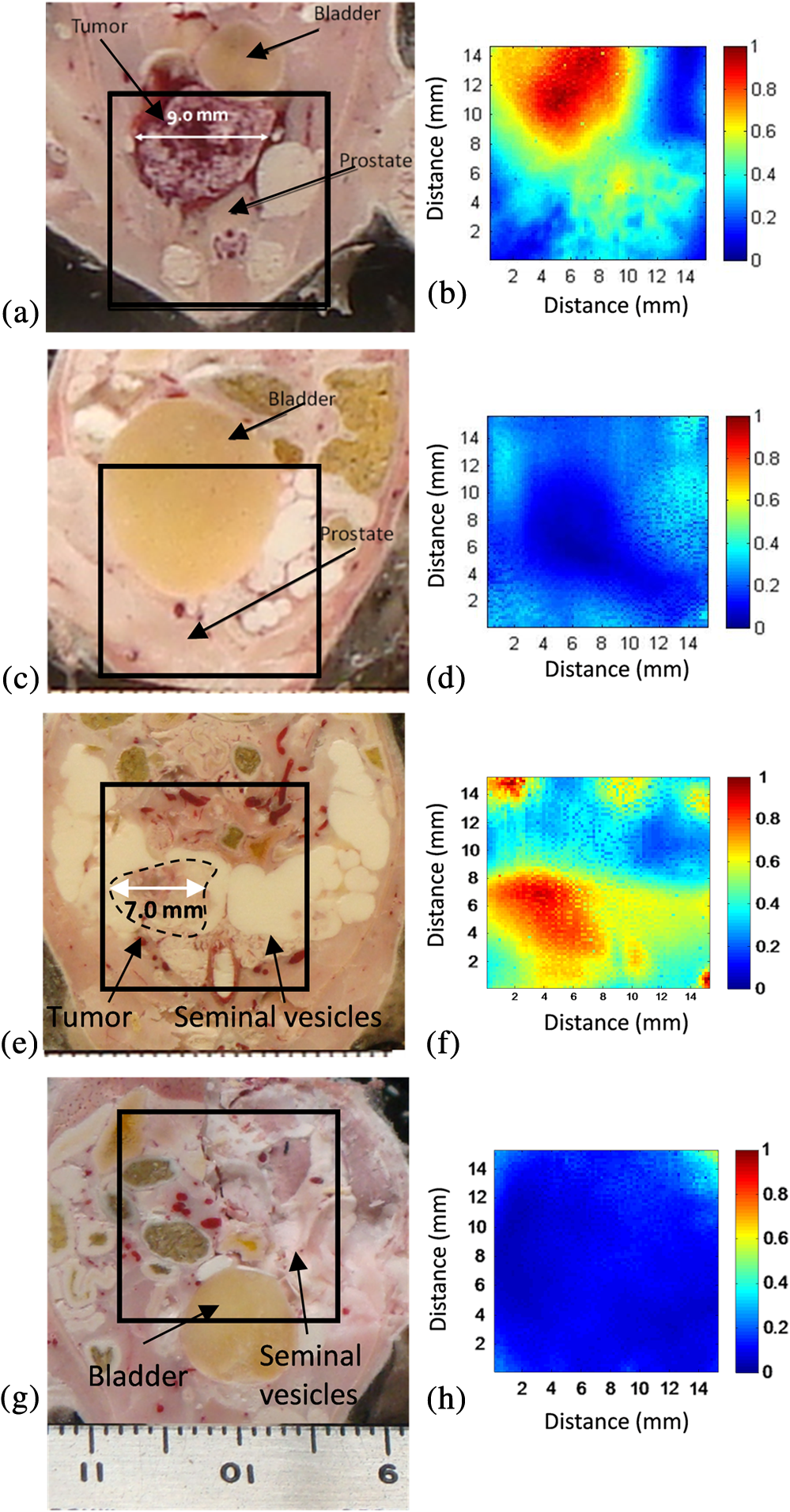

OA contrast for tumor compared to adjacent normal, healthy tissue ranged from 31 to 36 dB across the five TRAMP mice (Table 1). The OA contrast for the tumor compared to the region of the prostate on the age-matched control animal also ranged from 31 to 36 dB. The uncertainties of the contrast values are one standard deviation of the values measured within the boundaries of the ROI_analysis in the OA image.

Table 1

OA image contrast for five TRAMP mice and age-matched controls, and lateral TRAMP tumor dimensions.

Animal #	Contrast (dB)		Lateral dimension (mm)
Animal #	Tumor—adjacent	Tumor—control	From OA image	From cryosection
1	$33 \pm 2$	$34 \pm 2$	8.8	9.0
2	$31 \pm 2$	$35 \pm 2$	7.0	7.0
3	$33 \pm 2$	$36 \pm 2$	6.0	6.5
4	$36 \pm 2$	$34 \pm 2$	5.6	6.0
5	$31 \pm 2$	$31 \pm 2$	8.0	8.0

The OA predicted maximum lateral tumor dimension determined using the FWHM approach and the dimensions determined from the cryosections for the five TRAMP mice are summarized in Table 1. True tumor dimensions were measured during cryosectioning using a ruler. Tumor dimensions (measured on cryosections) ranged from 6.0 to 9.0 mm. The results show that the OA predicted tumor dimensions agree with the cryosection tumor dimensions to within 0.5 mm in all five TRAMP mice.

3.2.

Frequency Spectrum Analysis

A representative calibrated and noncalibrated power spectra for one OA dataset are shown in Fig. 3. A linear fit was applied to the normalized spectrum between 1 and 6 MHz.

Fig. 3

Representative power spectrums. (a) Uncalibrated RF tissue spectrum and calibration spectrum of the 5 MHz transducer. (b) The calibrated tissue power spectrum and linear fit applied between 1 and 6 MHz.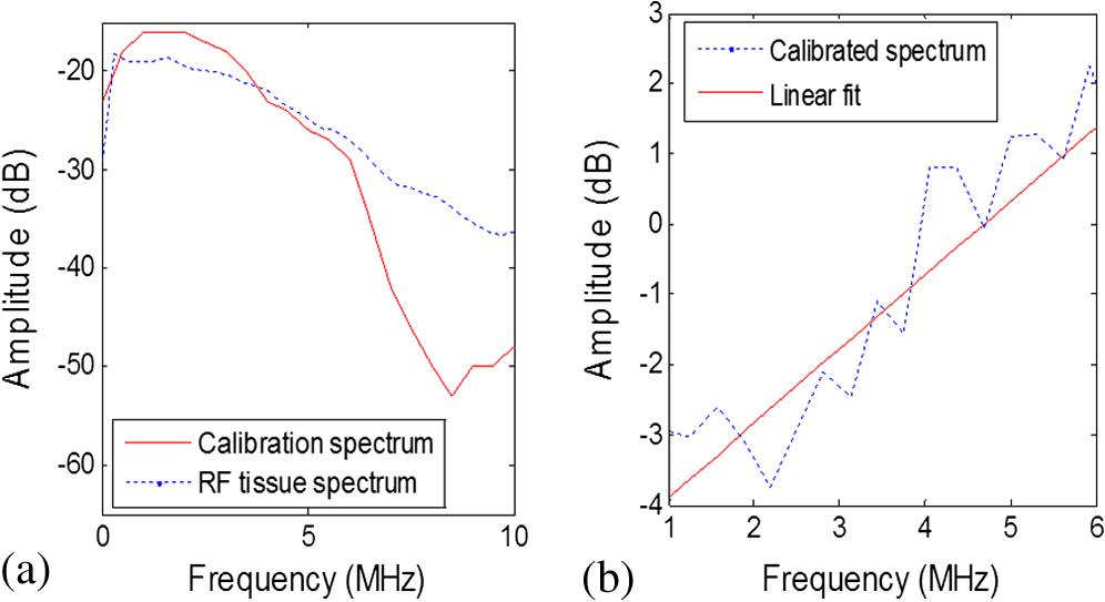

The midband fit, intercept, and slope values for the five TRAMP mice and age-matched controls are presented in Fig. 4 and Table 2. The data in Fig. 4 represent an average of 100 spectral parameter values acquired within a $2 \times 2 \times 2 mm$ ROI for all five mice. Error bars represent one standard deviation. Tumor tissues generate higher values of all three components compared with normal tissues (adjacent and control).

Fig. 4

Spectral components on tumor and adjacent to tumor for each TRAMP mouse and age-matched control mouse. Midband fit (a), intercept (b), and slope (c). Each value represents an average of spectral parameters acquired within a $2 \times 2 \times 2 mm$ region of interest.

Table 2

Average standard deviations of spectral components on tumor and adjacent to tumor for all TRAMP and for all control mice (N=5).

Spectral parameter	Control	Adjacent	Tumor	$t$ -test ( $p$ value)
Spectral parameter	Control	Adjacent	Tumor	tumor/control	tumor/adjacent
OA midband fit (dB)	$- 5 \pm 1$	$- 5 \pm 1$	$1 \pm 1$	0.0114	0.0040
OA slope (dB/MHz)	$0.4 \pm 0.1$	$0.4 \pm 0.1$	$0.8 \pm 0.1$	0.0026	$< 0.001$
OA intercept (dB)	$- 7 \pm 2$	$- 8 \pm 1$	$- 3 \pm 1$	0.0155	$< 0.001$

Note: OA, optoacoustic.

Mean and standard deviation values from all TRAMP mice on the tumor and on the adjacent tissue from all the control mice are presented in Table 2. There is a six-fold increase in midband fit and a two-fold increase in slope values on the tumor compared with the control. Significant differences ( $p < 0.05$ ) were found between all spectral components. No significant difference was found between the control and the adjacent spectral parameter values.

Cross-sectional profiles of the slope across the lateral dimension of a TRAMP tumor and age-matched control are shown in Fig. 5. Slope values are independent of signal strength (provided the SNR is adequate) and would remove the need to correct for optical attenuation. Therefore, analyzing slope values may be a more robust method of identifying tumor boundaries. The image shows that there is a gradual increase in slope values from the boundaries of the tumor to the center and variations within the tumor.

Fig. 5

Representative slope (dB/MHz) values across the lateral direction through a tumor in the TRAMP model (red) and in the control animal (blue). Vertical lines represent the boundaries of the tumor obtained from FWHM measurements on the OA amplitude images.

4. Discussion

The goal of this study was to demonstrate the potential of OA imaging to distinguish neoplastic prostate tissue in a transgenic tumor model from normal tissue in a control model. The amplitude and RF frequency components of the OA signals showed significant differences between cancerous and normal tissues. The results may arise from the principle that the amplitude of the OA signal is largely affected by the optical absorption of the target (determined by, e.g., blood vessel size, oxygenation status), while the frequency component may be more related to the geometrical properties of absorbing structures (e.g., blood vessel size, oxygenation status, and spatial distribution).³²

Our imaging approach of integrating OA signals within a 3 μs time window and projecting these values onto a 2-D plane yielded OA images with tumor contrast of 31 to 36 dB. The OA predicted dimensions agree with the true dimensions to within 0.5 mm. Further data from an increased number of animals may allow a more precise estimate of these variables to facilitate calibration of the OA data analysis.

The axial position of the front surface of the tumor in the OA image correlated to within 0.5 mm of the position measured during cryosectioning. The 2-D raster scan method of acquiring OA signals results in limited axial penetration depth due to the large optical attenuation in tissue (especially in tumor tissues due to elevated hemoglobin concentration).⁴³ To account for this optical attenuation, a depth dependent signal correction factor was applied to the OA signals prior to analysis.

Theoretical models relating the spectral intercept and slope for conventional ultrasound RF data and the tissue scattering structures have been well established.⁸^,²⁹ For conventional ultrasound imaging, the spectral components, slope, intercept, and midband fit are related to the physical characteristics of the target scatterer (e.g., the size, shape, acoustic impedance, and spatial distribution of the scatterering sources).⁸ The primary absorbing target for OA application in this paper is hemoglobin, which is localized in blood vessels.

The amplitude of the OA signal strongly affects the amplitude of the frequency spectrum, thereby affecting the midband fit and intercept values while the slope should be independent of amplitude (provided the signal-to-noise is adequate).⁴⁷ The OA signal amplitude is depth dependent due to high optical attenuation in tissues. For example, tumors with similar OA characteristics but positioned at different depths may yield different midband and intercept values. Hence, correcting for changes in fluence for variable target (i.e., tumor) depths is important. The depth dependent signal correction applied to the OA signals in this study represents an initial approach toward accounting for the optical attenuation. Significant differences between spectral parameters were found with and without the correction factor (data not shown).

Differences in spectral components of neoplastic tissue compared with healthy tissue have been reported for ultrasound RF data.⁴⁸ Neoplastic tissues have a different microstructure than that of healthy tissue; for example, neoplastic tissues are often denser than normal tissue and consist of more tortuous vasculature.⁴⁹ This leads to significant differences in the spectral components associated with neoplastic tissue compared to many healthy tissues.⁵⁰

Poorly differentiated prostate tumors are characterized by smaller vessels with greater microvessel density.⁵¹ Additionally, the aggressiveness of the tumor has been associated with the vessel diameter and microvessel density,⁵¹^,⁵² which has been demonstrated to be indicative of the chances of cancer survival for several malignancies.⁵³

A similar spectrum analysis technique for OAs has been reported by Kumon et al. who found a significant increase in the midband fit between on and off tumor but no significant differences for the intercept and slope.⁵⁴ Kumon et al. found midband fit values were 8.8 dB higher on the tumor compared with adjacent normal tissue. Similarly, we found midband fit values were 6 dB higher on the tumor compared with adjacent tissue. The slope values presented by Kumon et al. were $0.5 dB / MHz$ higher on the tumor (with no significant difference between the tumor and normal) compared with the slope values of this study, which were $0.4 dB / MHz$ higher on tumor tissue and significantly different from normal tissue. Our study demonstrates significant differences in all three spectral parameters between on and off tumor. Furthermore, control animals were used in this study to ensure that the OA signals adjacent to the tumor were consistent with normal tissues and not affected by the presence of the tumor.

The cross-sectional profile of the slope across a TRAMP tumor (Fig. 5) shows a gradual increase in the slope across the tumor boundary. Slope values are independent of signal strength (provided the SNR is adequate) and would remove the need to correct for optical attenuation. Therefore, analyzing the slope values may be a more robust method of identifying tumor boundaries.

OA imaging has shown promising initial results for detecting the presence of cancerous tumors with high contrast and good resolution compared with conventional ultrasound imaging.¹⁰^,¹⁴^,¹⁵ Using frequency spectrum analysis in combination with the current amplitude presentation of OA images may offer potentially important information about the tumor (e.g., vascular density, diameter, etc.). In a clinical setting, OA imaging (amplitude presentation) may be used to detect the presence of a tumor and its position in the tissue/organ. The frequency analysis of the RF signals from this tumor could then be performed to obtain further information on its physiological properties that may be indicative of its aggressiveness and treatability. Typical qualitative OA images, using only signal amplitude information, are also subject to a variety of user- and system-dependent factors (e.g., brightness/contrast, thresholding, laser fluence, etc.) that make it difficult to compare between studies. Frequency analysis described herein removes many of these factors by compensating for the system response and correcting for loss in optical fluence with depth.

The effective acquisition time of this system, $\sim 1 Hz$ , is due to the existing firmware. Future work will involve decreasing this delay time to optimize imaging time while minimizing any detection of the signal generated by previous pulses.

Additional studies including a larger number of animals are required to validate the contrast between the tumor, the preneoplastic tissue, and the healthy prostate as presented in this paper and to determine the optimal analysis techniques for image generation and boundary determination. A framework for understanding how spectral features are related to tissue physiology will need to be established along with statistical methods for classifying different tissues.²⁹ OA imaging of prostate tumors obtained at varying time points may also demonstrate the capability of these analysis techniques to not only detect the presence of the tumor but to also give an indication of the extent of the disease.

5. Conclusions

This study reports that there are significant differences between the amplitude and frequency content of OA signals between a tumor and healthy tissue. The increased signal amplitude is due to the increased vascularization within the tumor. The differences in the frequency components, however, are likely due to the combination of increased vascularization and vascular heterogeneity (more tortuous and smaller vessels size) of tumor tissues compared to healthy tissues. Frequency analysis, unlike amplitude analysis, of OA signals provides information about nonresolvable vascular structures, an important consideration since many OA imaging systems cannot resolve individual blood vessels at the depth of the prostate.²⁷^,²⁸ Knowledge of these vascular characteristics may aid in cancer diagnosis and treatment planning. This report has demonstrated the utility of standard pulse-echo spectrum analysis techniques for OA characterization of normal and neoplastic tissues. The results of this work contribute to the growing evidence-based support for optoacoustics as a cancer imaging tool.

Acknowledgments

The authors would like to gratefully acknowledge financial support provided by the Atlantic Canada Opportunities Agency, the Natural Sciences and Engineering Research Council of Canada, Innovation Prince Edward Island, and the Canada Foundation for Innovation. This research was undertaken, in part, thanks to funding from the Canada Research Chairs Program awarded to M. Kolios and W. Whelan. The authors also thank Dr. J. Spears and M. Arsenault from the Atlantic Veterinary College for technical support with the animal experiments.

References

1.

E. El-Gabryet al., “Imaging prostate cancer: current and future applications,” Oncology, 15 (3), 325 –336 (2001). 47AIAP 0030-2414 Google Scholar

2.

T. Liuet al., “A feasibility study of novel ultrasonic tissue characterization for prostate-cancer diagnosis: 2D spectrum analysis of in vivo data with histology as gold standard,” Med. Phys., 36 (8), 3504 –3511 (2009). http://dx.doi.org/10.1118/1.3166360 MPHYA6 0094-2405 Google Scholar

3.

R. D. Philipp Dahm, Evidence-Based Urology, 245 –250 Wiley, Hoboken, New Jersey (2010). Google Scholar

4.

J. Swanevelder, “Resolution in ultrasound imaging,” Contin. Educ. Anaesth. Crit. Care Pain, 11 (5), 186 –192 (2011). http://dx.doi.org/10.1093/bjaceaccp/mkr030 1743-1816 Google Scholar

5.

H. WijkstraM. H. WinkR. de la, “Contrast specific imaging in the detection and localization of prostate cancer,” World J. Urol., 22 (5), 346 –350 (2004). http://dx.doi.org/10.1007/s00345-004-0419-7 WJURDJ 0724-4983 Google Scholar

6.

B. TurkbeyP. A. PintoP. L. Choyke, “Imaging techniques for prostate cancer: implications for focal therapy,” Nat. Rev. Urol., 6 (4), 191 –203 (2009). http://dx.doi.org/10.1038/nrurol.2009.27 NRNADQ 1759-4812 Google Scholar

7.

M. H. Robert Ross, “New clinical imaging modalities in prostate cancer,” Hematol./Oncol. Clin. North Am., 20 (4), 811 –830 (2006). http://dx.doi.org/10.1016/j.hoc.2006.03.009 HCNAEQ 0889-8588 Google Scholar

8.

E. J. Feleppaet al., “Recent developments in tissue-type imaging (TTI) for planning and monitoring treatment of prostate cancer,” Ultrason. Imaging, 26 163 –172 (2004). http://dx.doi.org/10.1177/016173460402600303 ULIMD4 0161-7346 Google Scholar

9.

L. L. Fredericet al., “Ultrasonic spectrum analysis for tissue evaluation,” Pattern Recognit. Lett., 24 (4–5), 637 –658 (2003). http://dx.doi.org/10.1016/S0167-8655(02)00172-1 PRLEDG 0167-8655 Google Scholar

10.

L. V. Wang, “Ultrasound-mediated biophotonic imaging: a review of acousto-optical tomography and photo-acoustic tomography,” Dis. Markers, 19 (2–3), 123 –138 (2004). http://dx.doi.org/10.1155/2004/478079 DMARD3 0278-0240 Google Scholar

11.

J. MamouM. L. Oelze, Quantitative Ultrasound in Soft Tissues, 350 Springer, New York, NY (2013). Google Scholar

12.

W.-F. CheongS. A. PrahlA. J. Welch, “A review of the optical properties of biological tissues,” IEEE J. Quantum Electron., 26 (12), 2166 –2185 (1990). http://dx.doi.org/10.1109/3.64354 Google Scholar

13.

B. LashkariA. Mandelis, “Comparison between pulsed laser and frequency-domain photoacoustic modalities: signal-to-noise ratio, contrast, resolution, and maximum depth detectivity,” Rev. Sci. Instrum., 82 (9), 94903 (2011). http://dx.doi.org/10.1063/1.3632117 RSINAK 0034-6748 Google Scholar

14.

R. O. EsenalievA. A. KarabutovA. A. Oraevsky, “Sensitivity of laser opto-acoustic imaging in detection of small deeply embedded tumors,” IEEE J. Sel. Top. Quantum Electron., 5 (4), 981 –988 (1999). http://dx.doi.org/10.1109/2944.796320 IJSQEN 1077-260X Google Scholar

15.

A. A. Oraevskyet al., “Laser optoacoustic imaging of the breast: detection of cancer angiogenesis,” Proc. SPIE, 3597 352 –363 (1999). http://dx.doi.org/10.1117/12.356829 PSISDG 0277-786X Google Scholar

16.

M. SarntinoranontF. RooneyM. Ferrari, “Interstitial stress and fluid pressure within a growing tumor,” Ann. Biomed. Eng., 31 (3), 327 –335 (2003). http://dx.doi.org/10.1114/1.1554923 ABMECF 0090-6964 Google Scholar

17.

J. Shahet al., “Photoacoustic imaging and temperature measurement for photothermal cancer therapy,” J. Biomed. Opt., 13 (3), 034024 (2008). http://dx.doi.org/10.1117/1.2940362 JBOPFO 1083-3668 Google Scholar

18.

Y. Laoet al., “Noninvasive photoacoustic imaging of the developing vasculature during early tumor growth,” Phys. Med. Biol., 53 (15), 4203 –4212 (2008). http://dx.doi.org/10.1088/0031-9155/53/15/013 PHMBA7 0031-9155 Google Scholar

19.

S. HuL. V. Wang, “Photoacoustic imaging and characterization of the microvasculature,” J. Biomed. Opt., 15 (1), 011101 (2010). http://dx.doi.org/10.1117/1.3281673 JBOPFO 1083-3668 Google Scholar

20.

C. ZhangK. MaslovL. V. Wang, “Subwavelength-resolution label-free photoacoustic microscopy of optical absorption in vivo,” Opt. Lett., 35 (19), 3195 –3197 (2010). http://dx.doi.org/10.1364/OL.35.003195 OPLEDP 0146-9592 Google Scholar

21.

J. Lauferet al., “Three-dimensional noninvasive imaging of the vasculature in the mouse brain using a high resolution photoacoustic scanner,” Appl. Opt., 48 (10), D299 –D306 (2009). http://dx.doi.org/10.1364/AO.48.00D299 APOPAI 0003-6935 Google Scholar

22.

J. Lauferet al., “In vivo longitudinal photoacoustic imaging of subcutaneous tumours in mice,” Proc. SPIE, 7899 789915 (2011). http://dx.doi.org/10.1117/12.876782 PSISDG 0277-786X Google Scholar

23.

R. K. Sahaet al., “Validity of a theoretical model to examine blood oxygenation dependent optoacoustics,” J. Biomed. Opt., 17 (5), 055002 (2012). http://dx.doi.org/10.1117/1.JBO.17.5.055002 JBOPFO 1083-3668 Google Scholar

24.

F. L. Lizziet al., “Theoretical framework for spectrum analysis in ultrasonic tissue characterization,” J. Acoust. Soc. Am., 73 (4), 1366 –1373 (1983). http://dx.doi.org/10.1121/1.389241 JASMAN 0001-4966 Google Scholar

25.

J. ZalevM. C. Kolios, “Detecting abnormal vasculature from photoacoustic signals using wavelet-packet features,” Proc. SPIE, 7899 78992M (2011). http://dx.doi.org/10.1117/12.873911 PSISDG 0277-786X Google Scholar

26.

T. L. Hallet al., “Acoustic access to the prostate for extracorporeal ultrasound ablation,” J. Endourol., 24 (11), 1875 –1881 (2010). http://dx.doi.org/10.1089/end.2009.0567 JENDE3 0892-7790 Google Scholar

27.

M. XuL. Wang, “Photoacoustic imaging in biomedicine,” Rev. Sci. Instrum., 77 041101 (2006). PHYSGM 1943-2879 Google Scholar

28.

K. H. SongL. V. Wang, “Deep reflection-mode photoacoustic imaging of biological tissue,” J. Biomed. Opt., 12 (6), 060503 (2007). http://dx.doi.org/10.1117/1.2818045 JBOPFO 1083-3668 Google Scholar

29.

F. L. Lizziet al., “Ultrasonic spectrum analysis for tissue assays and therapy evaluation,” Int. J. Imaging Syst. Technol., 8 (1), 3 –10 (1997). http://dx.doi.org/10.1002/(ISSN)1098-1098 IJITEG 0899-9457 Google Scholar

30.

M. Kolios, “Biomedical ultrasound imaging from 1 to 1000 MHz,” Can. Acoust., 37 (3), 35 –43 (2009). CAACDX 0711-6659 Google Scholar

31.

F. L. Lizziet al., “Statistical framework for ultrasonic spectral parameter imaging,” Ultrasound Med. Biol., 23 (9), 1371 –1382 (1997). http://dx.doi.org/10.1016/S0301-5629(97)00200-7 USMBA3 0301-5629 Google Scholar

32.

G. J. DieboldA. C. BeveridgeT. J. Hamilton, “The photoacoustic effect generated by an incompressible sphere,” J. Acoust. Soc. Am., 112 (5 Pt 1), 1780 –1786 (2002). http://dx.doi.org/10.1121/1.1508788 JASMAN 0001-4966 Google Scholar

33.

A. G. Gertschet al., “Toward characterizing the size of microscopic optical absorbers using optoacoustic emission spectroscopy,” Proc. SPIE, 7564 75641M (2010). http://dx.doi.org/10.1117/12.844188 PSISDG 0277-786X Google Scholar

34.

R. H. Silvermanet al., “Spectral parameter imaging for detection of prognostically significant histologic features in uveal melanoma,” Ultrasound Med. Biol., 29 (7), 951 –959 (2003). http://dx.doi.org/10.1016/S0301-5629(03)00907-4 USMBA3 0301-5629 Google Scholar

35.

J. R. Gingrichet al., “Pathologic progression of autochthonous prostate cancer in the TRAMP model,” Prostate Cancer Prostatic Dis., 2 (2), 4096 –4102 (1999). http://dx.doi.org/10.1038/sj.pcan.4500296 PCPDFW 1365-7852 Google Scholar

36.

J. R. Gingrichet al., “Metastatic prostate cancer in a transgenic mouse,” Cancer Res., 56 (18), 4096 –4102 (1996). CNREA8 0008-5472 Google Scholar

37.

M. H. Enget al., “Early castration reduces prostatic carcinogenesis in transgenic mice,” Urology, 54 (6), 1112 –1119 (1999). http://dx.doi.org/10.1016/S0090-4295(99)00297-6 0090-4295 Google Scholar

38.

S. B. Shappellet al., “Prostate pathology of genetically engineered mice: definitions and classification. The consensus report from the bar harbor meeting of the mouse models of human cancer consortium prostate pathology committee,” Cancer Res., 64 (6), 2270 –2305 (2004). http://dx.doi.org/10.1158/0008-5472.CAN-03-0946 CNREA8 0008-5472 Google Scholar

39.

K. Passleret al., “Piezoelectric annular array for large depth of field photoacoustic imaging,” Biomed. Opt. Express, 2 (9), 2655 –2664 (2011). http://dx.doi.org/10.1364/BOE.2.002655 BOEICL 2156-7085 Google Scholar

40.

American National Standard for the safe use of lasers/secretariat, The Laser Institute of America, The Institute, Orlando, Florida (1993). Google Scholar

41.

L. Xiet al., “Photoacoustic imaging based on MEMS mirror scanning,” Biomed. Opt. Express, 1 (5), 1278 –1283 (2010). http://dx.doi.org/10.1364/BOE.1.001278 BOEICL 2156-7085 Google Scholar

42.

B. Coxet al., “Quantitative spectroscopic photoacoustic imaging: a review,” J. Biomed. Opt., 17 (6), 061202 (2012). http://dx.doi.org/10.1117/1.JBO.17.6.061202 JBOPFO 1083-3668 Google Scholar

43.

M. R. Arnfieldet al., “Optical properties of experimental prostate tumors in vivo,” Photochem. Photobiol., 57 (2), 306 –311 (1993). http://dx.doi.org/10.1111/php.1993.57.issue-2 PHCBAP 0031-8655 Google Scholar

44.

A. de la Zerdaet al., “Ultrahigh sensitivity carbon nanotube agents for photoacoustic molecular imaging in living mice,” Nano Lett., 10 (6), 2168 –2172 (2010). http://dx.doi.org/10.1021/nl100890d NALEFD 1530-6984 Google Scholar

45.

L.-S. Bouchardet al., “Picomolar sensitivity MRI and photoacoustic imaging of cobalt nanoparticles,” Proc. Natl. Acad. Sci. U. S. A., 106 4085 –4089 (2009). http://dx.doi.org/10.1073/pnas.0813019106 PNASA6 0027-8424 Google Scholar

46.

E. Strohmet al., “Photoacoustic spectral characterization of perfluorocarbon droplets,” Proc. SPIE, 8223 82232F (2012). http://dx.doi.org/10.1117/12.906042 PSISDG 0277-786X Google Scholar

47.

R. Silvermanet al., “Fine-resolution photoacoustic imaging of the eye,” Proc. SPIE, 7564 75640Y (2010). http://dx.doi.org/10.1117/12.842471 PSISDG 0277-786X Google Scholar

48.

J. Mamouet al., “Original contribution: three-dimensional high-frequency backscatter and envelope quantification of cancerous human lymph nodes,” Ultrasound Med. Biol., 37 345 –357 (2011). http://dx.doi.org/10.1016/j.ultrasmedbio.2010.11.020 USMBA3 0301-5629 Google Scholar

49.

J. Folkman, “Tumor angiogenesis: therapeutic implications,” New Engl. J. Med., 285 (21), 1182 –1186 (1971). http://dx.doi.org/10.1056/NEJM197108122850711 NEJMAG 0028-4793 Google Scholar

50.

B. Banihashemiet al., “Ultrasound imaging of apoptosis in tumor response: novel preclinical monitoring of photodynamic therapy effects,” Cancer Res., 68 (20), 8590 –8596 (2008). http://dx.doi.org/10.1158/0008-5472.CAN-08-0006 CNREA8 0008-5472 Google Scholar

51.

N. Weidneret al., “Tumor angiogenesis and metastasis—correlation in invasive breast carcinoma,” New Engl. J. Med., 324 (1), 1 –8 (1991). http://dx.doi.org/10.1056/NEJM199101033240101 NEJMAG 0028-4793 Google Scholar

52.

D. HanahanJ. Folkman, “Patterns and emerging mechanisms of the angiogenic switch during tumorigenesis,” Cell, 86 (3), 353 –364 (1996). http://dx.doi.org/10.1016/S0092-8674(00)80108-7 CELLB5 0092-8674 Google Scholar

53.

L. A. MucciA. PowolnyE. Giovannucci, “Prospective study of prostate tumor angiogenesis and cancer-specific mortality in the health professionals follow-up study,” J. Clin. Oncol., 27 (33), 5627 –5633 (2009). http://dx.doi.org/10.1200/JCO.2008.20.8876 JCONDN 0732-183X Google Scholar

54.

R. E. KumonC. X. DengX. Wang, “Frequency-domain analysis of photoacoustic imaging data from prostate adenocarcinoma tumors in a murine model,” Ultrasound Med. Biol., 37 (5), 834 –839 (2011). http://dx.doi.org/10.1016/j.ultrasmedbio.2011.01.012 USMBA3 0301-5629 Google Scholar

Biographies of the authors are not available.

CC BY: © The Authors. Published by SPIE under a Creative Commons Attribution 4.0 Unported License. Distribution or reproduction of this work in whole or in part requires full attribution of the original publication, including its DOI.

Citation Download Citation

Michelle P. Patterson, Christopher B. Riley, Michael C. Kolios, and William M. Whelan "Optoacoustic characterization of prostate cancer in an in vivo transgenic murine model," Journal of Biomedical Optics 19(5), 056008 (9 May 2014). https://doi.org/10.1117/1.JBO.19.5.056008

Published: 9 May 2014

Access the abstract

JOURNAL ARTICLE
8 PAGES

DOWNLOAD PAPER SAVE TO MY LIBRARY

GET CITATION

CITATIONS

Cited by 22 scholarly publications.

Explore citations on Lens.org

KEYWORDS

Tumors

Tissues

Control systems

Signal attenuation

Prostate

Prostate cancer

Ultrasonography

1.

Introduction

2.

Materials and Methods