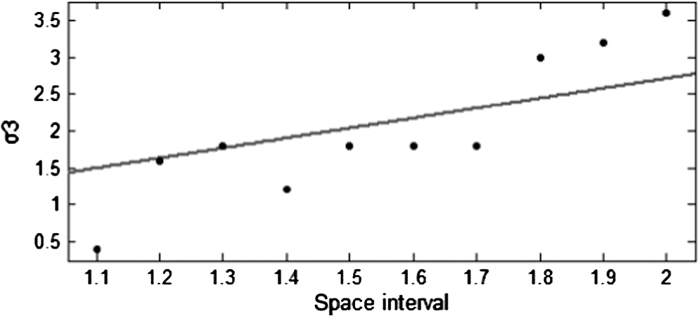
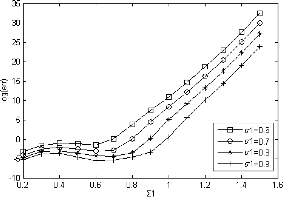
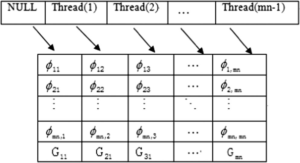
1.

Introduction

Various factors such as diffraction and aberration of optical systems could cause certain degradations in the microscopic imaging of biological specimens; such degradations are specifically known as image blurring or distortion.

The point spread function (psf) model directly influences the imaging process of biological specimens. Gaussian function is the most common and widely used psf model in many optical measurements and imaging systems. In these systems, the psf model is determined by various factors, but the synthesized result of all factors always makes the psf tend to be a Gaussian type. Currently, related researches on Gaussian psf model mainly focus on the identification of parameter $\sigma$, which is also known as the standard deviation of Gaussian function. A method proposed in the literature¹ makes use of a property of the Gaussian function and the Gaussian scale space representation of an image to identify $\sigma$. Another exploration is to select the maximum point of the differential coefficients of restored image Laplacian ${\mathrm{L}}_1$-norm curve.²

The classical deconvolution algorithms for microscopic images are on the basis that the psf is known or accurately measured or computed beforehand. According to different deconvolution principles, these algorithms could be generally divided into linear methods,^3,4 filtering methods,⁵ statistical methods,⁶ etc. However, under many conditions, the psf is often unknown or time-variant, which requires conducting a blind deconvolution process in the absence of priori knowledge. For either of the classical or blind deconvolution algorithms, the image and psf are usually expressed as discrete regular grid models in spatial or frequency domain. On occasions such as superresolution analysis or high-resolution image restoring based on a large set of data, since the image data always have a great correlation or redundancies, including steps of quantitative discrete convolutional or Fourier transform operations, the pure discrete grid models are usually quite time-consuming and not so efficient to optimize the whole deconvolution process. Due to the Gaussian type tendency of the psf in most microscopic systems, a new deconvolution method based on the Gaussian radial basis function (GRBF) interpolation is proposed in this paper. Both the original image and the psf are expressed as the same continuous GRBF model; thus image degradation is simplified as convolution of two continuous Gaussian functions, and image deconvolution is converted to calculate the weighted coefficients of two-dimensional (2-D) control points. Keeping consistent and concise continuous representation form during the whole course of restoring with no time-consuming discrete operations of convolution or Fourier transform, the whole deconvolution process can be easily optimized and controlled by computerized algorithms based on the introduced GRBF interpolation model; thus the defect of common discrete grid model mentioned above can be avoided.

Actually, the process of image deconvolution is quite time-consuming; in order to meet the needs of practical application, for both the discrete and continuous models, the implementation of specific algorithm inevitably involves some acceleration methods which include optimizing and simplifying the algorithm and adopting the multithreaded, distributed hardware architecture, etc. In recent years with the high-speed development of graphic processing unit (GPU), general purpose computing on GPU (GPGPU) has been widely used. Launched in 2007 by NVIDIA company, compute unified device architecture (CUDA) makes GPGPU more promising. There are a few reports^7,8 using CUDA to accelerate the incremental Wiener filter and Lucy–Richardson (LR) algorithm, respectively, in fields of microscopic and astronomical image deconvolution. For the implementation of the proposed GRBF method in this paper, CUDA will be adopted to accelerate parts with an intensive computing such as calculating the weighted coefficients of control points and resampling the restored image.

2.

GRBF Deconvolution Method

If the optical system is linear shift-invariant, the degradation procedure of imaging can be mathematically described as

2.1.

Continuous Gaussian Modeling

With a single parameter, the 2-D normalized Gaussian psf can be written in the form below:

Eq. (2)

$$h(x,y,{\sigma }_1)=\frac{1}{2\pi {\sigma }_1^2}{e}^{-\frac{x^2+y^2}{2{\sigma }_1^2}},$$

where parameter ${\sigma }_1$ is a standard deviation which determines the shape of Gaussian psf.

For a $d$-dimension function $\mathrm{\Phi }$ defined in domain $x\in R^d$, the function space spanned by linear combination of all $\mathrm{\Phi }(x,x_j)$ is called RBF space in which $\mathrm{\Phi }(x-x_j)=\mathrm{\Phi }(\Vert x-x_j\Vert )$. As long as $\{x_j\}$ is different from each other, $\{\mathrm{\Phi }(x-x_j)\}$ is linearly independent. When all $\{x_j\}$ is distributed evenly in whole span of $R^d$, the linear combination of $\{\mathrm{\Phi }(x-x_j)\}$ can approximate almost any function.⁹

2-D GRBF is described as

Eq. (3)

$$\varphi (\Vert {x-x}_i\Vert ,\Vert y-y_j\Vert ,{\sigma }_2)=e^{(-\frac{\Vert x-x_i{\Vert }^2+\Vert y-y_j{\Vert }^2}{2{\sigma }_2^2})},$$

where $\Vert ·\Vert$ denotes Euclidean norm, $(x_i,y_j)$ is the 2-D coordinate of control points, and ${\sigma }_2$ is the parameter of GRBF.

A set of basis functions ${\{\varphi (x-x_i,y-y_j,{\sigma }_2)\}}_{j=0,i=0}^{m-1,n-1}$ are obtained through translating control points, then the original 2-D image can be expressed as continuous Gaussian model $f(x,y,{\sigma }_2)$ by GRBF interpolation

Eq. (4)

$$f(x,y,{\sigma }_2)=\sum _{j=0}^{m-1}\sum _{i=0}^{n-1}{a}_{i,j}·\varphi (\Vert x-x_i\Vert ,\Vert y-y_j\Vert ,{\sigma }_2),$$

where $m$ and $n$ denote the number of 2-D control points in vertical and horizontal directions, respectively, and $a_{i,j}$ are the weighted coefficients. Through GRBF interpolation, the original image is represented in accord with the psf expression form, thus the process of image degradation can be simplified as the weighted sum of convolution of two continuous Gaussian functions according to the deduction in

Eq. (5)

$$\begin{gathered} f(x,y,{\sigma }_2)·h(x,y,{\sigma }_1)={\int }_{-\infty }^{+\infty }{\int }_{-\infty }^{+\infty }f(x,y,{\sigma }_2)·h(x-u,y-v,{\sigma }_1)\mathrm{d}u\mathrm{d}v \\ ={\int }_{-\infty }^{+\infty }{\int }_{-\infty }^{+\infty }(\sum _{j=0}^{m-1}\sum _{i=0}^{n-1}{a}_{i,j}·e^{-\frac{{(x-x_i)}^2+{(y-y_j)}^2}{2{\sigma }_2^2}})·\frac{1}{2\pi {\sigma }_1^2}·e^{-\frac{{(x-u)}^2+{(y-v)}^2}{2{\sigma }_1^2}}\mathrm{d}u\mathrm{d}v \\ =\frac{1}{2\pi {\sigma }_1^2}·\sum _{j=0}^{m-1}\sum _{i=0}^{n-1}{a}_{i,j}·({\int }_{-\infty }^{+\infty }{\int }_{-\infty }^{+\infty }{e}^{-\frac{{(x-x_i)}^2+{(y-y_j)}^2}{2{\sigma }_2^2}}·e^{-\frac{{(x-u)}^2+{(y-v)}^2}{2{\sigma }_1^2}}\mathrm{d}u\mathrm{d}v) \\ =\frac{1}{2\pi {\sigma }_1^2}·\sum _{j=0}^{m-1}\sum _{i=0}^{n-1}{a}_{i,j}·\frac{2\pi {\sigma }_1^2{\sigma }_2^2}{{\sigma }_1^2+{\sigma }_2^2}·e^{-\frac{{(x-x_i)}^2+{(y-y_j)}^2}{2({\sigma }_1^2+{\sigma }_2^2)}} \\ =\frac{{\sigma }_2^2}{{\sigma }_3^2}·\sum _{j=0}^{m-1}\sum _{i=0}^{n-1}{a}_{i,j}·e^{-\frac{{(x-x_i)}^2+(y-y{}_j)^2}{2{\sigma }_3^2}}, \end{gathered}$$

where ${\sigma }_3^2={\sigma }_1^2+{\sigma }_2^2$ is the standard deviation of new Gaussian function. Substituting Eq. (5) into Eq. (1), the process of image degradation can be described as

Eq. (6)

$$g(x,y)=\frac{{\sigma }_2^2}{{\sigma }_3^2}·\sum _{j=0}^{m-1}\sum _{i=0}^{n-1}{a}_{i,j}·e^{-\frac{{(x-x_i)}^2+{(y-y_j)}^2}{2{\sigma }_3^2}}+n(x,y).$$

Equation (6) shows that the blurred image $g(x,y)$ is still a continuous GRBF interpolation model. Let discrete blurred image data ${\{(p,q),G_{p,q}\}}_{q=0,p=0}^{M-1,N-1}\in (N^2,R)$ satisfy $g(p,q)=G_{p,q}$, where $(p,q)$ is the 2-D coordinate of blurred image $G$, and $M$ and $N$ denote the height and width of the blurred image, respectively. Thus the process of image deconvolution is actually converted to a problem of calculating $a_{i,j}$. The computing complexity of continuous GRBF interpolation model shown in Eq. (6) is only decided by the space interval or the number of control points. Therefore, the whole process of image deconvolution can easily be globally optimized by simply setting the space interval or the number of control points.

The value of ${\sigma }_3$ directly affects the interpolation accuracy. Along with ${\sigma }_3$ increasing, the shape parameter $1/2{\sigma }_3^2$ of GRBF becomes smaller, as a result, the GRBF is becoming relatively flat. When GRBF is made too flat, obvious instability will appear in the process of interpolation, that is to say, there exists large vibration in $a_{i,j}$ magnitude. There are two methods named Contour-Pade/SVD¹⁰ and RBF-QR¹¹ reported to effectively solve the instability of flat RBF interpolation, but both expose their inherent limitations. In this paper, we try to increase the space interval, i.e., reducing the number of control points (normally the number of control points is equal to or less than the number of image pixels) to solve the instability problem. But increasing the space interval of control points will inevitably lead to the decline of accuracy in restored images; the selection of space interval should be appropriate to make a trade-off between interpolation stability and deconvolution accuracy.

Before establishing the relationship between ${\sigma }_3$ and space interval, we define the mean square error (MSE) as

Eq. (7)

$$\mathrm{MSE}=\frac{1}{MN}·\sum _{j=0}^{M-1}\sum _{i=0}^{N-1}{[g(i,j)-\widehat{g}(i,j,{\sigma }_3)]}^2,$$

where $\widehat{g}(i,j,{\sigma }_3)$ is the interpolation image of $g(i,j)$. Then a series of experiments are performed based on various value combinations of the space interval and ${\sigma }_3$, where the experimental space interval begins at 1.0 and ends in 2.0 with a step length of 0.1; meanwhile, taking 0.2 as a step length, ${\sigma }_3$ begins at 0.2 and ends in 6.0.

Figure 1 shows that in the case of $\text{space}\text{interval}=1.0$, ${\sigma }_3=2.0$ is the critical point of interpolation stability, the MSE is nearly 0 when ${\sigma }_3\le 2.0$, yet MSE sharply increases and vibrates when ${\sigma }_3>2.0$. Analyzing a single curve under the condition of “$\text{space}\text{interval}>1.0$,” it is found that MSE is very large when ${\sigma }_3<1.0$, which means the interpolation is instable; then MSE becomes small and the curve keeps relatively flat as ${\sigma }_3$ changes in the range of 1.0 to 3.0; finally, MSE increases gradually when ${\sigma }_3>3.0$. By selecting the ${\sigma }_3$ that corresponds to the minimum value of MSE, the “space interval–${\sigma }_3$” line is fitted.

Fig. 1

The ${\sigma }_3$-MSE curves with different space intervals.

In Fig. 2, the slope of the fitted line is 1.356 with 95% confidence interval (1.068, 1.644). Figures 1 and 2 show that increasing the space interval of control points can effectively solve the problem of interpolation instability caused by flat GRBF (when space interval is equal to 1.0 and ${\sigma }_3>2.0$). Finally, the relational expression between ${\sigma }_3$ and space interval is obtained

Eq. (8)

$${\sigma }_3=\{\begin{array}{ll}R,R\in (0,2],& \text{space}\text{interval}=1\\ 1.356\text{space}\text{interval},& \text{space}\text{interval}\in (1,2]\end{array}.$$

Fig. 2

The space interval $-{\sigma }_3$ fitted line.

2.2.

Deconvolution with ${\sigma }_1$ and ${\sigma }_2$

The previous section introduces a method by increasing the space interval of control points to solve the problem of interpolation instability. However, the quality of restored image is influenced by the interaction of ${\sigma }_1$ and ${\sigma }_2$, where ${\sigma }_1$ is the parameter of continuous Gaussian psf model $h(x,y,{\sigma }_1)$, and ${\sigma }_2$ is the parameter of original image continuous GRBF model $f(x,y,{\sigma }_2)$.

The whole calculations for deconvolution of large size images will burden the computer very much and cause an inconceivable time overhead due to the massive GRBF data. Therefore, it is necessary to evenly divide the large size image into several subimages with small size, then put all the restored subimages together, while main computation is finished. But the quality of the restored image will decline because of white artifact lines produced in the joints of restored subimages. The solution is to let adjacent subimages keep a overlapping region from each other, where the size of the overlapping region is decided according to the $3\sigma$ principle of Gaussian function, then utilize a suture algorithm¹² among the overlapping regions of restored subimages

Eq. (9)

$$I_{\text{new}}=I_{\text{left}}·(1-\mathrm{coef})+I_{\text{right}}·\mathrm{coef},$$

where $I_{\text{new}}$ is the synthesized image part of overlapping regions, $I_{\text{left}}$ and $I_{\text{right}}$ are the left and right regions of $I_{\text{new}}$, respectively, and coef is a weighted factor. The simplest way is to set $\mathrm{coef}=0$ in $I_{\text{left}}$ and $\mathrm{coef}=1$ in $I_{\text{right}}$.

Assuming the blurred image $g(x,y)$ with a dimension size of $512\times 512$ is divided into several $26\times 26$ size subimages, every subimage keeps an overlap of 5 pixels with the adjacent ones. When ${\sigma }_1$ is known, the ${\sigma }_2-\log (\mathrm{MSE})$ curves are shown in Fig. 3, where MSE calculates the MSE between original image $f(x,y)$ and restored image $\widehat{f}(x,y,{\sigma }_1,{\sigma }_2)$, and the negative value in $\widehat{f}(x,y,{\sigma }_1,{\sigma }_2)$ is constrained to 0. It can be found from Fig. 3(a) when $\text{space}\text{interval}=1.0$ and ${\sigma }_1$ is equal to 0.8, 1.0, 1.2, 1.4, and 1.6, respectively, each of the curves exists an obvious feature point, where ${\sigma }_2$ corresponds to 1.9, 1.7, 1.6, 1.5, and 1.6, respectively. The curve segment on the left side of each feature point is strictly monotone decreasing, and at each feature point the curve has a minimum value (except ${\sigma }_1=1.6$), the curve segment on the right side of each feature point begins to vibrate. According to the equation ${\sigma }_3^2={\sigma }_1^2+{\sigma }_2^2$, ${\sigma }_3$ is obtained. The corresponding ${\sigma }_3$ is equal to 2.0616, 1.9723, 2.0000, 2.0518, and 2.2627, respectively, which just locates around the critical point of interpolation stability in Fig. 1. When ${\sigma }_1=0.8$, ${\sigma }_1=1.0$, or ${\sigma }_1=1.2$, the corresponding ${\sigma }_2$ of feature point is larger than ${\sigma }_1$ and log(MSE) is smaller than 0, which means the restored image has a good quality. When ${\sigma }_1=1.4$ or ${\sigma }_1=1.6$, the corresponding ${\sigma }_2$ of feature point is close to ${\sigma }_1$ and log(MSE) is large, which means the restored image has a relatively big error compared with the original image. Increasing the space interval can effectively improve the quality of restored image when ${\sigma }_1$ is large. Figure 3(b) shows the ${\sigma }_2-\log (\mathrm{MSE})$ curves when space interval is equal to 1.2. There also exist feature points, where ${\sigma }_2$ corresponds to 1.5, 1.7, 1.8, 2.0, and 2.3, respectively. The curve segment on the left side of each feature point is steep, while on the right side the curve segment keeps more flat. The corresponding ${\sigma }_2$ of each feature point is larger than ${\sigma }_1$, and the corresponding ${\sigma }_3$ is equal to 1.7000, 1.9723, 2.1633, 2.4413, and 2.8018, respectively, which locates in the middle segment of the curve in Fig. 1.

Fig. 3

${\sigma }_2-\log (\mathrm{MSE})$ curves with different ${\sigma }_1$. (a) $\text{Space}\text{interval}=1.0$. (b) $\text{Space}\text{interval}=1.2$.

Through the comparison between Figs. 3(a) and 3(b), it can be concluded that when ${\sigma }_1$ is small, the corresponding log(MSE) of each feature point in Fig. 3(a) is smaller than that in Fig. 3(b); when ${\sigma }_1$ is large, the corresponding log(MSE) of each feature point in Fig. 3(b) is smaller than that in Fig. 3(a). Moreover, in both cases the corresponding ${\sigma }_2$ is larger than ${\sigma }_1$.

When psf parameter ${\sigma }_1$ is unknown, the estimated value will greatly affect the quality of restored image. An estimation or identification method is provided below. Based on the continuous GRBF interpolation model, the grayscale range of restored image and original image is quite close if only the estimated value ${\mathrm{\Sigma }}_1$ is smaller than or equal to the true ${\sigma }_1$. However, the grayscale range of restored image broadens obviously when ${\mathrm{\Sigma }}_1$ is larger than ${\sigma }_1$. As a result, more large negative values appear in the restored image. Under this circumstance, the true ${\sigma }_1$ can be better estimated. The estimated criterion is defined as

Eq. (10)

$$\mathrm{err}=\frac{1}{MN}·\sum _{j=0}^{M-1}\sum _{i=0}^{N-1}{(g(i,j,{\sigma }_1)-h({\mathrm{\Sigma }}_1)·|\widehat{f}(i,j,{\sigma }_2,{\mathrm{\Sigma }}_1)|)}^2,$$

where $g(i,j,{\sigma }_1)$, $h({\mathrm{\Sigma }}_1)$, and $\widehat{f}(i,j,{\sigma }_2,{\mathrm{\Sigma }}_1)$ represent blurred image, psf, and restored image, respectively. When ${\sigma }_1$ is small, a collection of candidates is provided (${\mathrm{\Sigma }}_1$ begins at 0.2 and ends in 1.5 with a step length of 0.1). By setting $\text{space}\text{interval}=1.0$ and ${\sigma }_2=1.0$, the relationship curves are plotted in Fig. 4.

Fig. 4

${\mathrm{\Sigma }}_1-\log (\mathrm{err})$ curves with different ${\sigma }_1$.

Figure 4 shows that when ${\sigma }_1$ is equal to 0.6, 0.7, 0.8, and 0.9, respectively, the curves exist obvious feature points, where ${\mathrm{\Sigma }}_1$ corresponds to 0.6, 0.7, 0.8, and 0.9, respectively. The curve segment on the left side of each feature point has small log(err), while on the right side of each feature point, the log(err) increases sharply. The corresponding ${\mathrm{\Sigma }}_1$ of each feature point is the optimal estimation of ${\sigma }_1$. When ${\sigma }_1$ is large enough, it is needed to set $\text{space}\text{interval}>1.0$ and ${\sigma }_2>{\sigma }_1$. Although the ${\mathrm{\Sigma }}_1$ that corresponds to the point of $\log (\mathrm{err})=0$ is close to ${\sigma }_1$, there exists no obvious feature point due to the influence of ${\sigma }_2$ selection and the loss of interpolation accuracy. In this case, Eq. (10) is only suitable as a preliminary estimated criterion.

2.3.

GPU Parallel Computing

Based on the continuous GRBF interpolation model, the microscopic image deconvolution requires a large amount of computation; therefore, it is unable to meet the real-time requirement. There are two effective ways used to speed up the computation. One is to increase the space interval of control points, which will cause a loss of deconvolution accuracy. Another is to adopt the multithreaded programming model without the loss of deconvolution accuracy. Considering the data distribution is regular in the process of calculating weighted coefficients of control points and resampling the restored image, CUDA can take full advantage of GPU multiprocessors to achieve the goal of real-time implementation for the microscopic image deconvolution.

Without considering the influence of noise $n(x,y)$, Eq. (6) is expressed as a discrete form of matrix multiplication

Eq. (11)

$$G=\frac{{\sigma }_2^2}{{\sigma }_3^2}·\mathrm{\Phi }\times A.$$

Let the number of control points $m$ and $n$ be equal to the height $M$ and width $N$ of image, respectively; $\mathrm{\Phi }$ is a $mn$-by-$mn$ GRBF symmetric matrix; $G$ is a $mn$-by-1 blurred image column matrix. According to Eq. (11), the process of calculating weighted coefficient matrix $A$ is mathematically to solve a large system of linear equations, the general methods for solving linear equations include direct method and iterative method. Since matrix $\mathrm{\Phi }$ is not diagonally dominant, the matrix $A$ calculated by iterative method¹³ is divergent.

In order to reduce the time overhead and meet the requirement of coalesced access¹⁴ in CUDA, the column-based Gaussian elimination method is adopted. Figure 5 takes $c=1$ as an example, where $c$ is the label of column. Threads $1,2,\dots$ and $mn-1$ are in charge of the elimination between the column of ${\varphi }_{11}$ and the columns of ${\varphi }_{12},{\varphi }_{13},\dots$ and ${\varphi }_{1,mn}$, respectively, as a result, ${\varphi }_{12},{\varphi }_{13},\dots$ and ${\varphi }_{1,mn}$ are eliminated to 0. Because these threads access to the adjacent location in global memory, in a warp, threads only execute one access; therefore, it greatly reduces the memory access overhead. CPU controls to repeat a total of ($mn-1$) elimination loops, ($mn-c$) threads are needed in each elimination loop. Finally, $\mathrm{\Phi }$ is eliminated to be a left triangular form, then matrix $A$ can be calculated by using back-substitution.

Fig. 5

Diagram of parallel column-based Gaussian elimination method.

In the process of large size image deconvolution, if all the subimages use column-based Gaussian elimination method to calculate matrix $A$, the cumulative time is still very long. We can combine matrix $\mathrm{\Phi }$ with identity matrix $E$, and use parallel column-based Gauss–Jordan elimination method¹⁵ to calculate the inverse matrix ${\mathrm{\Phi }}^{-1}$. Then each matrix $A$ is calculated by ${\mathrm{\Phi }}^{-1}\times G$, which also needs to meet the requirement of coalesced access.

The continuous GRBF model of restored image is obtained by putting the weighted coefficients of control points into Eq. (4). Each pixel resampling only relates to its position coordinate and the weighted coefficients of control points. Thus, the procedure can set multiple threads; each thread solely executes a pixel resampling.

3.

Experiments and Results

The conventional objective evaluation criteria of a restored image mostly evaluate the whole image in the spatial domain,¹⁶ which cannot effectively distinguish between the high-frequency component and low-frequency component of the restored image. In this paper, a frequency objective evaluation criterion is adopted. The mean of frequency spectrum (MFS) is defined as

In order to prove the efficiency of image deconvolution, the GRBF method is compared with Wiener filter and LR algorithm. Based on the stationary random process, Wiener filter is an ideal deconvolution method that minimizes the MSE between original image and restored image. LR algorithm¹⁷ is an iterative method based on Bayesian analysis, this algorithm has the unique solution when the influence of noise can be ignored or is very small.

In our simulation experiments, CPU is AMD Sempron 140 and GPU is NVIDIA GTX 680 with 1536 stream processors, the software platforms are MATLAB 2012b and CUDA, respectively. The original image is a $512\times 512$ size mice cochlea laser scanning confocal microscope image. In order to analyze every spectrum range, the MFS of each concentric circle that takes the position of $\widehat{F}(0,0)$ as a common center and $r$ as the radius is calculated.

First, the original image is degraded by Gaussian psf of ${\sigma }_1=1.2$. LR algorithm runs 50 iterations. $\mathrm{GRBF}(t_1,t_2)$ indicates that the size of subimage is $t_1\times t_2$, herein $t_1$ and $t_2$ have not included the overlapping pixels. The optimal space interval and ${\sigma }_2$ are set to be 1.0 and 1.6, respectively, according to Fig. 3, and the adjacent subimages keep an overlap of 6 pixels. It can be seen in Fig. 6, along with the increase of radius $r$, frequency spectrum transits from low-frequency spectrum to high-frequency spectrum, and the amplitude of spectrum gradually decreases. When $r<30$, the MFS of the blurred image is basically equal to the MFS of the restored image, which means image deconvolution has little change on the low-frequency component. As $r$ increases, within each spectrum range, the MFS of GRBF method is larger than the MFS of Wiener filter or LR algorithm, which means the GRBF method can better increase the high-frequency component and improve the clarity of the restored image. By comparing the MFS of GRBF(16,16) and GRBF(32,32) method, it is found that the two $r$-MFS curves almost overlap together, which means the size of the subimage has limited impact on the quality of the restored image.

Fig. 6

r-MFS curves.

The MSE of GRBF method is smaller than the MSE of Wiener filter or LR algorithm, and the MFS of GRBF method is larger than the MFS of Wiener filter or LR algorithm as shown in Table 1. The two objective evaluation criteria indicate that the image restored by GRBF method is clearer and much closer to the original image. However, the running time of GRBF method is much longer.

Table 1

Comparison of the results of mice cochlea images implemented on CPU.

Figure 7(b) is the blurred image degraded by Gaussian psf of ${\sigma }_1=1.2$, Figs. 7(c)–7(e) are the images restored by Wiener filter, LR algorithm, and GRBF(16,16) method, respectively. In order to conveniently display the image, Fig. 7 only shows the $128\times 128$ size areas picked from the $512\times 512$ size images. From appearance, the image clarity of GRBF method is successively higher than the image clarity of LR algorithm and Wiener filter.

Fig. 7

Comparison of mice cochlea images. (a) The original image. (b) The blurred image degraded by Gaussian psf of ${\sigma }_1=1.2$. (c) The image restored by Wiener filter. (d) The image restored by LR algorithm. (e) The image restored by GRBF(16,16) method.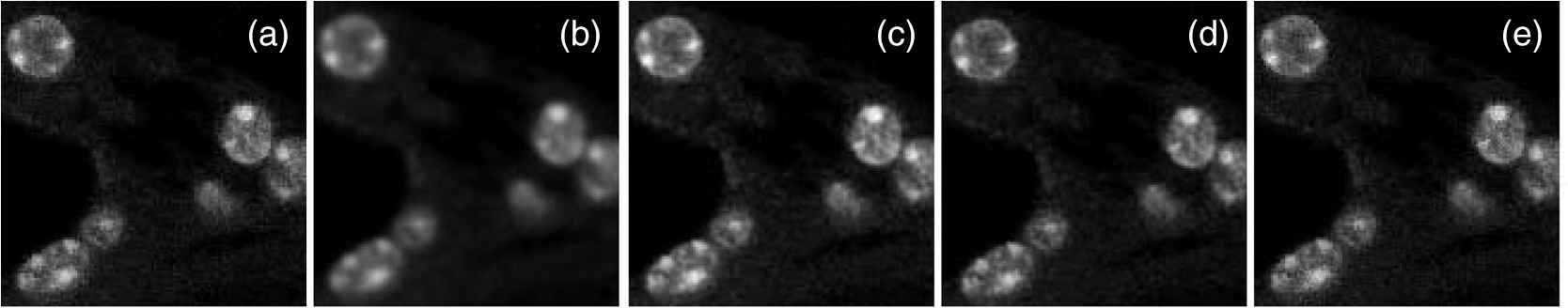

Based on GPU multithreaded programming model, CUDA can greatly accelerate the implementation of the GRBF method.

The MSE and MFS calculated on GPU change little compared with the results calculated on CPU, and the running time is reduced to 1.2600 and 5.9620 s, respectively, as shown in Table 2. It is important to note because the ${\sigma }_3$ is at the critical point of interpolation stability in Fig. 1, single-precision floating point calculations of the GRBF method will bring a great error; therefore, the program must adopt double-precision floating point calculations.

Table 2

The results of GRBF method implemented on GPU.

Since the original image is expressed as a continuous Gaussian model, we can easily scale the restored image. Table 3 shows the results of resampled images with different sizes. As size increases, the running time is mainly consumed in image resampling. CUDA can obviously accelerate the implementation of resampling. Take the $2048\times 2048$ size resampled image as an example: the speedup ratio can exceed 110 times. As size increases, it is found that MFS gradually decreases, which indicates that increasing the size will inevitably bring a certain degree of blurring in the resampled image.^18,19

Table 3

Comparison of the results among different size mice cochlea images resampled by GRBF(16,16) method.

Another effective way to reduce the running time is to increase the space interval of control points, which will cause a loss of deconvolution accuracy. In Table 4, the original image is still degraded by Gaussian psf of ${\sigma }_1=1.2$. According to Secs. 2.1 and 2.2, the ${\sigma }_2$ should be larger than ${\sigma }_1$, and ${\sigma }_3$ needs to satisfy Eq. (8). When $\text{space interval}>1.0$, the upper bound limit of 95% confidence interval is selected to be the slope of fitted line; therefore, the calculation formula of ${\sigma }_2$ is

Table 4

Comparison of the results of GRBF(16,16) method with different space intervals.

As space interval increases, the running time gradually reduces, but the deconvolution accuracy also gradually declines, specifically, the MSE gradually increases and MFS gradually decreases.

It is seen from Fig. 8, although the clarity of the restored image gradually declines, it is higher than the clarity of the blurred image.

Fig. 8

Comparison of mice cochlea images. (a) The original image. (b) The blurred image degraded by Gaussian psf of ${\sigma }_1=1.2$. (c) The image restored by GRBF(16,16) method with $\text{space}\text{interval}=1.2$. (d) The image restored by GRBF(16,16) method with $\text{space}\text{interval}=1.6$. (e) The image restored by GRBF(16,16) method with $\text{space}\text{interval}=2.0$.

In order to test and verify whether the GRBF deconvolution method can still be applied to other microscopic images that have different characteristics. Figures 9 and 10 show the relative simulation results of mice tibial organ and mice kidney tissue images, respectively.

Fig. 9

Comparison of mice tibial organ images. (a) The original image. (b) The blurred image degraded by Gaussian psf of ${\sigma }_1=1.2$. (c) The image restored by Wiener filter. (d) The image restored by LR algorithm. (e) The image restored by GRBF(16,16) method.

Fig. 10

Comparison of mice kidney tissue images. (a) The original image. (b) The blurred image degraded by Gaussian psf of ${\sigma }_1=1.2$. (c) The image restored by Wiener filter. (d) The image restored by LR algorithm. (e) The image restored by GRBF(16,16) method.

The size of the experimental images are still $512\times 512$; Figs. 9(b) and 10(b) are the blurred image degraded by Gaussian psf of ${\sigma }_1=1.2$. In the process of GRBF deconvolution, it is found that ${\sigma }_3=2.0$ is still the critical point of interpolation stability when $\text{space}\text{interval}=1.0$. According to Secs. 2.1 and 2.2, the optimal ${\sigma }_2$ is selected to be 1.6. It is seen from Figs. 9 and 10 that the contrast in restored images obtained by three deconvolution methods is all enhanced, and the structure of mice tissue is clear. The data given in Tables 5 and 6 indicate that the images restored by the GRBF method are richer in high-frequency component and closer to the original images than the images restored by Wiener filter or LR algorithm.

Table 5

Comparison of the results of mice tibial organ images implemented on CPU.

Table 6

Comparison of the results of mice kidney tissue images implemented on CPU.

Figure 11 and Table 7 show the experimental results of $256\times 256$ size Derenzo phantom images; the procedure is as the same as that in microscopic image deconvolution. It can be seen in Figs. 11(c) and 11(d) that dot artifacts will appear in the round holes of Derenzo phantom images that restored by Wiener filter or LR algorithm, while the image restored by the GRBF method in Fig. 11(e) has no such dot artifacts.

Fig. 11

Comparison of Derenzo phantom images. (a) The original image. (b) The blurred image degraded by Gaussian psf of ${\sigma }_1=1.2$. (c) The image restored by Wiener filter. (d) The image restored by LR algorithm. (e) The image restored by GRBF(16,16) method.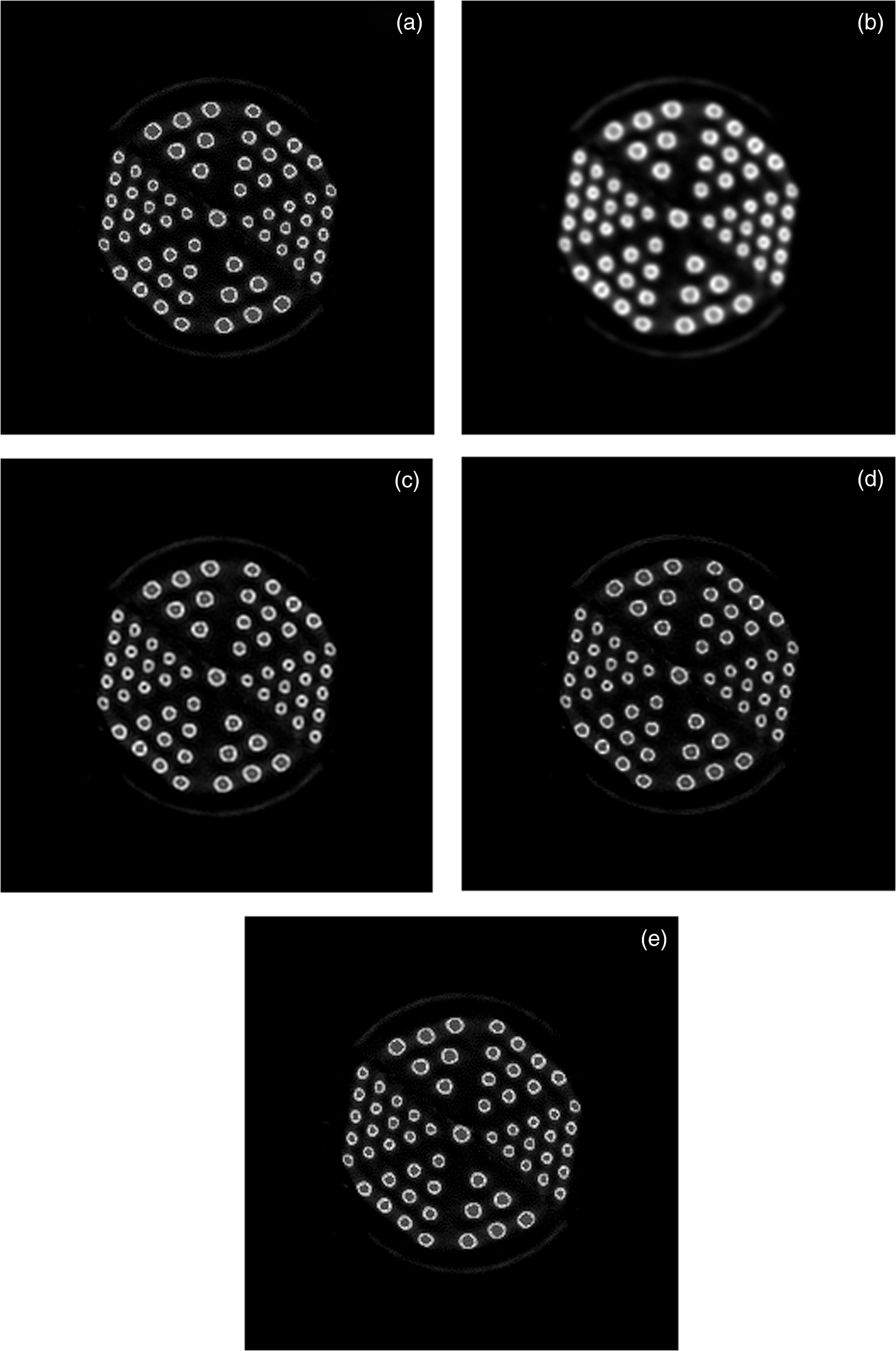

Table 7

Comparison of the results of Derenzo phantom images implemented on CPU.

4.

Conclusion

This paper presents a deconvolution method that expresses the blurred image $g(x,y)$, original image $f(x,y)$, and psf $h(x,y)$ as continuous models by using GRBF interpolation. On this basis, the process of image deconvolution is to calculate the weighted coefficients of control points and resample the restored image. The deconvolution accuracy and computing scale are greatly optimized by selecting the proper parameters. Compared with Wiener filter and LR algorithm, the GRBF method exposes advantages in the quality of the restored image. In addition, CUDA can effectively accelerate the implementation of the GRBF method.

In future research, the GRBF method can also be applied to three-dimensional (3-D) microscopic image deconvolution. Further studies are needed for efficiently expressing the 3-D psf,²⁰ effectively arranging the control points and properly selecting the GRBF expression²¹ in 3-D microscopic image deconvolution.