
|
|
1.IntroductionDiffuse reflectance spectroscopy (DRS), which encompasses techniques with more specific designations, including elastic scattering spectroscopy and light scattering spectroscopy, has demonstrated high value in recent years relevant to the goal of diagnosing disease in vivo1,2 in a wide range of organs, such as brain,3 cervix,4 skin,5 colon,6 breast,7 esophagus,8 pancreas,9 and oral cavity.10 Most commonly, DRS entails the transmission of broadband light [anywhere from near-UV through visible to near-IR (NIR)] through a fiberoptic probe to a turbid medium; after propagating through the sample, a fraction of the light is collected at the surface as reflectance, at a specified distance from the source entry point. Figure 1 illustrates a commonly employed probe geometry, with one fiber used for illumination and a separate fiber for collection. The measured reflectance spectrum can then be analyzed with appropriate mathematical models to extract the optical properties of the tissue, such as the reduced scattering and absorption coefficients ( and , respectively). These optical properties are directly determined by the cell morphology, the extracellular matrix, and the biochemistry and vascularization of the tissue, which undergo a predictable set of changes during the progression of disease.1 Thus, optical property differences are directly related to changes in the structural and biochemical tissue properties, and consequently, quantification of these optical properties can be used not only to inform about the tissue disease status, but also provide important contextual information about the physiological state of the tissue. The key, however, to reliable optical property quantification and disease classification using DRS is in the use of an accurate mathematical model to describe reflectance as a function of the optical properties of the tissue. Development of such reflectance models has been addressed using a variety of analytical and empirical approaches, which are sensitive to a range of parameters, including and , and the geometric specifications of the measurement probe. The description of reflectance as a function of optical property values was originally modeled using diffusion theory based on the diffusion approximation to the transport equation. 11 However, the use of diffusion theory is generally restricted to the conditions of the diffusion approximation: (1) scattering dominates absorption; and (2) the distance between the illumination and collection points is large compared to the mean-free-path for scattering. Except in the NIR spectral region, condition 1 is not generally met in tissue due to strong absorption by hemoglobin; and condition 2 (large source-detector separation) is often a limitation when accessing internal tissues or when highly localized tissue properties are sought. To avoid these restrictions, alternative models based on modifications to the diffusion theory, Monte Carlo simulations, or empirical formalisms from observation have been developed by various authors over the past 15 years.12–24 As with diffusion theory, however, these modified models only account for the relationship between reflectance and the scattering and absorption coefficients and generally do not account for other factors that are important for describing light reflectance under nondiffuse conditions. The importance of the scattering phase function (angular scattering probability distribution) is one such factor that is chronically overlooked, having been addressed for the incorporation into forward models by only a handful of authors.3,19,25,26 Further, most of these models have been developed for a single illumination-collection geometry, focusing either on very small source-detector separations () or on larger separations (of the order of several millimeters, approaching the diffusion regime), with less attention paid to intermediate distances. In this work, we present a generalized formalism that describes diffuse reflectance models for two-fiber collection geometries, such as that shown in Fig. 1, over a wide range of input parameters. This formalism provides an intuitive understanding of the trends concerning how reflectance is affected by tissue optical properties and by measurement geometries. In particular, we focus on the effects of the scattering phase function and the source-detector separation, , both of which are known to have strong influence on reflectance. The description of this generalized formalism builds upon previous work, which has explored expressions for reflectance as it relates these factors. We review and highlight how these previous observations all contribute and can be comprehensively understood within the scope of a single framework. In addition, we present several novel and significant observations that further enhance the understanding of the influence of the phase function and source-detector separation on reflectance models. These include the identification of a dimensionless scattering distance (within the nondiffuse regime) at which reflectance is insensitive to phase function, the use of a unique error-estimation approach to evaluate the accuracy of inverse property extraction (obtaining and estimates from in vivo reflectance measurements), and the demonstration of a simple method that allows for extraction of phase function information (in addition to and ) when analyzing reflectance measurements at two or more different source-detector separations. Taken as a whole, the trends and observations described in this work are intended to serve as a resource to better understand, from an intuitive perspective, how various input parameters can be expected to influence reflectance measurements, and the factors in probe geometry or experimental design that can enable the best performance for accurate retrieval of the desired tissue properties. Thankfully, with the recent advancement of graphical processing units (GPUs) for parallel computing, custom reflectance models can now be developed for a wide range of measurement geometries and tissue optical properties (including phase function) with relative ease. We begin with a comprehensive review of diffuse reflectance modeling and of phase function formalisms and trends specific to the optical characterization of tissue in Sec. 2. This is followed by a description of the Monte Carlo code and methods used for the investigation of reflectance relationships along with a description of the novel error-estimation approach for investigating the accuracy of inverse-model property extraction in Sec. 3. Section 4 presents the generalized reflectance framework that describes the relationships among reflectance values, optical property values (with particular emphasis on phase function), and source-detector separation. Inverse-model error analysis results are also presented and discussed. Previous contributions by others are clearly identified, as well as our own novel advancements. We conclude with key insights and recommendations concerning experimental design to minimize errors due to phase function uncertainty. 2.Background2.1.Modeling ReflectanceIn the context of DRS, a forward model is any function that quantitatively describes the relationships between measured reflectance and the multiple input parameters that will influence reflectance, such as the tissue optical properties and the geometry specifications of the optical measurement. The primary motivation for understanding these reflectance relationships is not for use in forward direction calculations, but rather for use in solving the inverse problem (calculating tissue optical properties from measured reflectance). The relationship between forward and inverse models is expressed generically in Eq. (1), where represents measured reflectance, is the scattering phase function, and represents all probe geometry parameters. 2.1.1.Forward modelThe forward model can be described in various ways either with analytical/empirical closed-form equations, or computationally using Monte Carlo simulations or look-up tables. Analytical forms include the diffusion theory equation and its many modified versions.11,13,16,26 Monte Carlo based reflectance models calculate reflectance using a single simulation, making use of similarity relationships to calculate reflectance for a large range of optical coefficients.24 Look-up tables, as their name implies, allow for calculation of reflectance by looking up a value based on a set of input optical parameters within a table of data collected from either phantoms or Monte Carlo simulated data.27 Empirical models use experimental data (again, either from phantoms or Monte Carlo simulated data) and fit it to a proposed closed-form equation that describes the data well.17–23,28 Several of these empirical models,23,28 including one developed by our group,22 describe the relationship between reflectance and optical property coefficients ( and ) using the framework of Beer’s Law, where reflectance under conditions of negligible absorption, , is scaled based on the absorption coefficient, , and the average photon path length, . Scattering-only reflectance, , is modeled to be a function of , and is modeled to be a function of and . The relationships describing and as functions of and contain constant coefficient values that are unique for a given optical probe geometry and tissue phase function, such that the model can be customized for a specific measurement probe.We note that, regardless of the specific form of the reflectance model (empirical, analytical, look-up table, etc.), as long as the description of each forward model represents the same reflectance relationships (reflectance versus optical property values) under the same geometry conditions, their performance in the inverse direction will be equivalent. Therefore, in this paper, we explore the dependence of reflectance models on the phase function and probe geometry from a general perspective. Relationships between reflectance and optical property values will be illustrated in a graphical format—reflectance as a function of or —with the understanding that this information can be converted into one of the other model formats as needed. (Empirical equations and lookup table formats provide the most flexibility for this purpose.) These graphical reflectance relationships form the basis of the generalized reflectance model formalism that is presented in Sec. 4. 2.1.2.Inverse modelBecause reflectance values are not uniquely associated with a single combination of scattering and absorption properties, using any model in the inverse direction is a fundamentally ill-posed problem and requires use of wavelength-dependent relationships for and to reduce the dimensionality of the problem. In models of tissue, the spectral shape of is often based on a power law,14,15,23,27 and the absorption coefficient is often determined by a linear combination of concentrations and extinction coefficients for oxyhemoglobin and deoxyhemoglobin [ and , respectively] sometimes with the addition of a correction for a vessel-packing factor, , to account for the fact that blood is confined within blood vessels rather than uniformly distributed.29,30 Thus, the tissue parameters can be represented as follows: where is a normalization wavelength. Here, , which is the absorption coefficient of whole blood, and are calculated as30 where is the concentration of hemoglobin in whole blood. Other contributions to the tissue absorption coefficient (e.g., beta carotene for adipose tissue in the visible, or water for any tissue in the NIR) can be added to as appropriate for the specific tissue and wavelength range. The remaining five coefficients include and , representing the scattering coefficient at a normalization wavelength, , and the scattering power-law exponent, related to average scatterer size, respectively, and , , and , representing the blood volume fraction (%), the hemoglobin oxygen saturation (%), and the average blood vessel radius, respectively. These wavelength relationships for and [Eqs. (3) and (4)] can then be substituted into any desired forward model. Measured reflectance spectra are fit to the model using a nonlinear least-squares curve fitting method, such as the Levenberg-Marquardt method, with , , , , and as the fitting coefficients. Thus, each measured spectrum can be characterized by these five physiological parameters. While these wavelength-dependent expressions for and are specific to tissue, by selecting alternative wavelength-dependent expressions, reflectance models can be used in the inverse direction to extract optical properties of any turbid medium.2.2.Phase FunctionsThe phase function, , of a scattering sample specifies the probability distribution of scattering angles and is typically normalized to 1, integrated over all solid angles. To generalize the phase function, the anisotropy factor, , is defined as the average cosine of the scattering angle, . In tissue, ranges, typically, between 0.75 and 0.99.31 The scattering coefficient, , and the anisotropy factor, , are often combined into a single parameter, known as the reduced scattering coefficient: . This similarity relationship is based on the assumed condition that observed optical measurements are equivalent for any combination of and that results in the same .32 Interest in the influence of the details of the phase function on reflectance measurements was originally reported by Mourant et al., Bevilacqua and Depeursinge, and Kienle et al., who demonstrated that reflectance is dependent on the specific form of phase function for reflectance measured close to the source ( source-detector separation in tissue), thus negating the applicability of the reduced scattering coefficient similarity condition for short distances.19,33,34 Bevilacqua and Depeursinge further explored the relationship between phase function and reflectance by considering higher moments of the phase function and by developing a new similarity relationship applicable for small source-detector separations.3,19 More recently, Kanick et al. have also utilized this similarity function for single-fiber source-detector geometries.35 In the derivation of the new similarity relationship, the phase function is expanded into a series of Legendre polynomials, where are the ’th-order Legendre moments. The first-order moment, , is equivalent to the familiar anisotropy factor, . To calculate its value from any arbitrary phase function, the following equation can be used:36 Similarly, using the second Legendre polynomial, , the second moment, , can be calculated as The calculations of and from Eqs. (5) and (6) assume that the phase function is already normalized, such that . From these two moments, the new similarity relationship and parameter is defined In the nondiffuse regime (i.e., when scattered light is detected after experiencing only a few scattering events), this additional parameter, , in addition to , helps to more accurately describe the scattering properties of a medium.19 Under these conditions, observed optical measurements will be equivalent for any combination of , , and , which result in the same values for and . From a physical perspective, is representative of the relative contribution of near-backward (large-angle) scattering in a phase function. The consideration of in quantitative reflectance models has been limited to an empirical model by Bevilacqua and Depeursinge, which employs multiple source-detector separations for use with radially resolved analysis,3,19 and more recently, a model for single-fiber reflectance measurement geometries by Kanick et al.35 Extending the work of these two groups, the generalized reflectance formalism presented in Sec. 4 examines the role of the parameter in reflectance models for two-fiber geometries over a broad range of separations.The use of is applicable to any phase function representation, including the commonly adopted Henyey-Greenstein (HG), modified HG (MHG), and more rigorous Mie theory formalisms, as described below. 2.2.1.Henyey-Greenstein and modified Henyey-GreensteinThe HG phase function is the most widely used function in the bio-optics community due to its simplified representation of tissue scattering.37 It is defined by the following equation: By selecting a given value, all other Legendre moments are automatically fixed: . Thus, the possible values for range from 1.0 to 2.0, as constrained by .From the few experimental studies on true effective phase functions in tissue, it has been observed that the HG phase function underestimates high-angle backward scattering.34,38,39 To address this drawback, a modified version of the HG function was proposed that combines the standard HG function with an added Rayleigh scattering component, which contributes additional high-angle scattering. Known simply as the MHG phase function, it is defined as where is the fractional contribution of the standard HG phase function, and conversely, is the fractional contribution of the Rayleigh scattering component.19 The first and second moments are easily calculated from the following: where is the value used to construct the HG phase function contribution from Eq. (6). With the added flexibility of the MHG phase function, both and can be controlled individually. Values of , however, are limited to the range of 1.0 to 2.0 due to mathematical constraints of the HG and MHG phase functions.2.2.2.Mie theory phase functionA more rigorous estimation of the phase function in tissue can be calculated from Mie theory by approximating tissue as a distribution of discretely sized spherical particles. By combining the individual phase functions from each sphere size, weighted by relative concentrations of different sizes, an average phase function can be constructed to represent the bulk medium. One proposed approach to selecting the appropriate sizes and distribution of particles to best approximate tissue is to use a fractal distribution, based on observations that refractive index variations measured by phase-contrast microscopy scale according to a power law.40–42 The number density, , of each particle size is then defined as where is the representative size of a spherical volume containing the particles, and is the fractal volume dimension that relates to the ratio of small versus large particles.40 A large value corresponds to a greater ratio of small to large particles.For each discrete particle size, Mie theory is used to calculate the scattering cross-section, , and the anisotropy factor, , using values for the medium and particle indices of refraction that are representative of cytoplasm () and cellular organelles (), respectively. Schmitt and Kumar calculated average values of and to 1.45.42 Using the assumption that waves scattered by individual particles add linearly, the anisotropy factor is defined as where is the total number of discrete particle sizes in the distribution.43,44 The combined phase function, , can be calculated from a linear combination of the scattering amplitude, (as defined by Bohren and Huffman in their formulation of Mie theory45), scaled by the number density of spheres. Calculation of and can then be performed using Eqs. (5) and (6).The use of Mie theory and the fractal distribution model of scattering sizes offers a unique opportunity to examine the relationship between and . Throughout this paper, calculations are performed using refractive index values and particle diameter values from the literature:42,43 , , , and a wavelength of . The fractal dimension, , is varied between 2 and 6, each value of corresponding to a unique pair of and . Different selections for , , , and the discrete particle sizes will yield slightly different numerical results for the relationship between and , but, in general, the trends remain the same. Figure 2 demonstrates that the relationship between and is nonlinear and that increases more rapidly for large values, especially when . This is especially important since most tissues have values in this higher range. Further, the values of in this region are generally (dependent on the values of , , , and ), which is the upper limit of for the HG and MHG phase functions, indicating that a phase function constructed from Mie theory is more appropriate when modeling tissue. Values of in tissue have been found to range from 1.7 to 2.2, which highlights the importance of using a phase function capable of values .3 Bevilacqua and Depeursinge have previously analyzed the space of possible combinations of values for , , and for various phase functions, noting the larger range of possible combinations for Mie phase functions as compared to HG and MHG.19 The analysis here differs by limiting the Mie phase functions to those constructed using the fractal particle distribution model, providing a simplified understanding of the relationship between and that is specifically representative of tissue. Fig. 2Relationship between the anisotropy values, and (for the specific parameters , , ), as calculated from Mie theory using a fractal distribution of scattering particle sizes () with the fractal dimension, , varied between 2 and 6. Differences in refractive index values and/or particle sizes will provide different numerical results, but the generalized shape of the curve will remain consistent.  For the purposes of comparison, Fig. 3 illustrates constructed functions for the HG, MHG, and Mie phase function descriptions. All three functions are for . However, the HG function has , while the MHG and Mie functions have values of , which can be seen in the differences in high-angle scattering between the HG function and the MHG and Mie functions. Note also that, despite having the same value, the MHG and Mie phase functions are not identical. Differences between the two result from, and can be observed in variations in the higher-order Legendre moments (). Fig. 3Comparison of a Henyey-Greenstein (HG), a modified Henyey-Greenstein (MHG), and a Mie phase function, all with , but with different values (HG: , MHG and Mie: ). 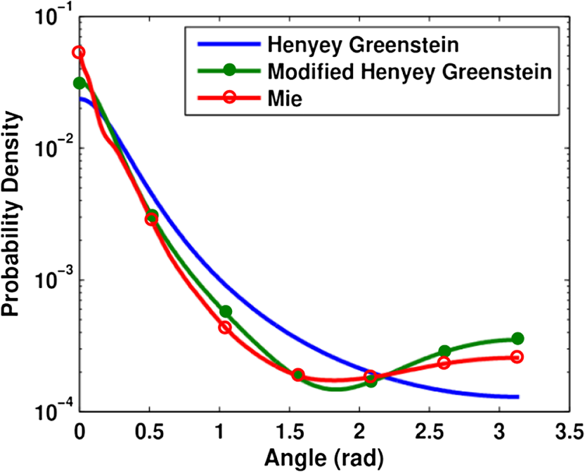 It is important to note that these phase functions are presented using the standard representation that specifies the distribution of light intensity scattered as a function of angle [], i.e., the relative power per unit solid angle that is observed at a given angle in a steady-state system. Alternatively, the phase function can be expressed as a probability distribution of scattering angles [], i.e., the probability that a photon will scatter at a given angle. The difference reflects the inherent field versus photon representation issue common in optics; the two forms are related as . In the literature, phase functions have been reported in both ways, without specifying which form is being used, which often leads to confusion.46,47 The angular representation, , needs to be used when sampling scattering direction changes in Monte Carlo simulations. 3.Methods3.1.Monte Carlo Simulations“Experimental” data for the work in this paper were obtained from Monte Carlo simulations. Computational simulation allows for a controlled and exact approach to the comparison of various models and input parameters, which would be more difficult experimentally using phantoms. A version of Monte Carlo for multilayered tissue48 adapted for use on a GPU was used for increased speed.49 This code was modified to launch and collect photons within the area and numerical aperture of user-defined fibers to model the two-fiber probe geometry (one illumination and one collection fiber), as illustrated in Fig. 1. Additionally, the code was modified to provide a choice in phase function, allowing the user to select , , , or any other user-defined phase function at run time. Monte Carlo simulations were run in sets, each having identical geometry and phase function input parameters. Table 1 reports the values of all input parameters used for the simulations. In each set, simulations were run for a set of combinations of reduced scattering coefficient values, , and absorption coefficient values, . For all simulations, constant values for the refractive index of the tissue, the refractive index of the fibers, the numerical aperture of the fibers, and the fiber diameter were used. All simulations were terminated upon the collection of 10,000 photons, such that the variances of the simulations were equivalent at according to Poisson statistics. Because of the equivalence of variances, and their small 1% value, error bars are not included on plots of results. Table 1Input parameters for Monte Carlo simulations. Parameters listed with an asterisk (*) are constant for all simulations.
To examine the effects of source-detector separation, sets of simulations were run for a range of values, . And for exploration of the effects of phase function, simulations were run assuming an MHG phase function form using various combinations of and . All combinations of the two variables were constructed, but due to the mathematical limitations of the form of the formula for MHG, phase function combinations with and and 0.85 are not possible and, thus, could not be simulated and evaluated. Mie theory–based phase functions were also considered, using constant refractive index values, particle sizes , and wavelength , while varying the fractal dimension, . Resulting anisotropy values of and were calculated using Eqs. (5), (6), (7), and (13). The values were selected such that the values of were spaced equally between 1.2 and 2.3; the range of was chosen to correspond to physiologically relevant anisotropy values between and 0.96 (see Fig. 2). The particle sizes and refractive index values are representative of tissue.42,43 While only two phase function models (MHG and Mie) were chosen here for analysis, note that regardless of the mathematical form of the phase function, the similarity relationship dictates that reflectance values will be equal for equal values of , and thus, the details of the higher-order moments of various models is not significant when considering reflectance model trends. Nonetheless, we note that only Mie theory can be invoked for values of . 3.2.Inverse Modeling: A Different Approach to Error AnalysisAs previously demonstrated in the literature,19,26,35 reflectance models depend on phase function, and hence, the choice of a model to use in the inverse direction requires knowledge of the tissue phase function. However, in most cases, this information is not known a priori and, consequently, assumptions must be made. An incorrect assumption will affect the accuracy of extracted scattering and absorption properties from measured reflectance; we wish to quantify the degree to which an incorrect assumption affects these extracted values. Unfortunately, because there is currently no gold standard for measuring the optical and physiological parameters from point measurements in tissue, it is not possible to experimentally test the effects of model differences. Therefore, the error analysis presented in this work uses computationally constructed reflectance data, which allows for a more controlled and exact approach to the comparison of various models and input parameters. This analysis first involves computationally constructing a set of reflectance spectra that are representative of the true model and tissue properties. Then the assumed reflectance model, which is different from the true model due to inaccurate assumptions about tissue phase function, is used in the inverse direction to extract the fitted optical property values. The differences between these extracted values and the actual property values, thus, provide a measure of error that represents the potential uncertainty in in vivo measurements. We note moreover, that this technique is novel in its approach to examining error in terms of extracted physiological values from reflectance spectra, as opposed to reporting error exclusively of the optical coefficient values. It is difficult to define a single estimate of error because the errors in extracted quantities are directly related to and themselves. Hence, errors are calculated for multiple reflectance spectra, each with different scattering and absorption properties. A set of wavelength-dependent and spectra are first calculated using Eqs. (3) and (4), over a wavelength range from 400 to at a resolution of 1 nm (for a total of 400 data points). Values for the five physiological fitting variables (, , , , and ) were selected such that the resulting and spectra would span the ranges characteristic of tissue. For scattering, four spectra were selected to represent overall low scattering (, ), medium scattering (, ), high scattering (, ), plus one with a large slope representing a high density of smaller scatterers (, ). The reference wavelength was selected to be 600 nm. For absorption, spectra were selected for a physically representative range of absorption values (blood volume fraction, , 2, and 5%), all with a moderate hemoglobin oxygen saturation level (). For all cases, the average blood vessel radius is held constant at which is representative of capillaries. Using all combinations of the scattering and absorption conditions, a set of 12 unique scattering and absorption spectra were used for testing. Computationally constructed reflectance spectra, representing measured data, are calculated using the test scattering () and absorption () spectra according to Eq. (1), where the forward reflectance model is specific to a single phase function [] and measurement geometry (). Reflectance values are calculated using the forward model via a lookup table composed of Monte Carlo simulated reflectance data specific to the unique pair of and . A bilinear interpolation algorithm (available in MATLAB®) was used to calculate reflectance values for combinations of and not explicitly listed in the table. Noise of 1% was added to the spectra to better represent experimentally acquired data. As previously mentioned, when using reflectance models in the inverse direction, the least-squares fitting algorithm is insensitive to the specific form of the forward model as long as the modeled reflectance is negligibly different over the set of and values. Hence, the choice of model format to use in the inverse direction can be based primarily on preference. For flexibility, we have chosen to use an interpolation lookup table method (with the same lookup table format used to construct the reflectance spectra). This is easily implemented in MATLAB® using the lsqcurvefit toolbox (using the Levenberg Marquardt optimization algorithm), as it can be constructed with any user-defined computational function for the forward model regardless of functional form. When calculating optical property extraction error associated with inaccuracies in phase function assumptions, reflectance spectra were calculated for all combinations of and spectra listed above, yielding a set of 12 reflectance spectra. The assumed reflectance model, representing an inaccurate choice of phase function, is then used in the inverse direction to fit each of the 12 true reflectance spectra and extract the fitting coefficients (, , , , and ) and, consequently, the and spectra. Errors in extracted optical and physiological values are reported as an average across all 12 combinations on a percentage basis for the physiological parameters (, , , , and ), and as the mean percentage error across the entire wavelength range for the optical coefficients ( and ). 4.Results and Discussion4.1.Phase Function DependenceMany reflectance models, specifically empirical models describing reflectance at small source-detector separations, have assumed an HG phase function with an anisotropy value .17,18,20,22 As introduced in Sec. 2.2, the MHG and the Mie phase functions have been shown in the literature to be more representative of true scattering in tissue as a consequence of the higher probability for large-angle scattering. To examine the impact of these phase functions that are more representative of tissue, specifically the influence of both and , reflectance relationships were simulated for a range of and values. The MHG phase function is user-friendly for this purpose, since it conveniently enables independent variation of and . Phase functions constructed using values of and described in Sec. 3.1 were examined using a source-detector separation of 250 μm. Figure 4 illustrates the resulting reflectance relationships when each of the phase functions is used for simulation. Fig. 4Reflectance relationship plots for a probe geometry with , and different MHG phase functions. Colors and symbols correspond to different values and line styles correspond to different g values. Note that plots for the combinations and and 1.9 are not present due to the mathematical limitations of the MGH phase function with these values.  In much of what follows, reflectance models are reported graphically in a set of two plots, as illustrated in Fig. 4. The left plot illustrates the relationship between the relative reflectance and the reduced scattering coefficient, , in the absence of absorption, and the right plot illustrates the relationship between reflectance and the absorption coefficient, . In the plot of reflectance versus , reflectance values are normalized to 1 at . This highlights the shape differences rather than the overall amplitude differences in reflectance, as caused by differences in . The two subplots correspond to the two components of the empirical model format inspired by Beer’s Law, presented in Eq. (2); the first represents Eq. (2) when such that , and the second represents Eq. (2) normalized such that . This graphical representation is useful for identifying trends, as it helps to distinguish the dependences of scattering and absorption separately. Most importantly, Fig. 4 reveals that when is held constant, the influence of is remarkably small. Conversely, when is held constant, reflectance values vary significantly with . At and , reflectance for is more than three times larger than for . Differences due to in the reflectance versus relationships are more moderate, but still show a significant dependence. This observation for a two-fiber geometry reflectance relationship follows from previous work by both Bevilacqua et al. and Kanick et al. (for radially resolved multifiber geometries and for single-fiber geometries) in that the critical phase function variable to consider when building reflectance models (for short source-detector distances) is , and not .3,19,35 We further emphasize not only that is more influential than , but also that the influence of is limited; phase functions with different values, but the same value, have reflectance relationships that are essentially similar. Because the MHG phase function is restricted to values , and yet Mie phase functions constructed to represent tissue have possible values , we also examined how Mie phase functions, which are more representative of tissue, influence reflectance relationships for an even wider range of . These results are presented in Fig. 5. As compared to the reflectance relationships built with the MHG phase function, the differences due to in the reflectance versus relationships are qualitatively similar. The differences in reflectance for the reflectance versus relationships, however, have increased such that, at , reflectance for is nearly six times larger than for . Further, as increases, the differences in reflectance become more substantial. For example, when considering values most representative of tissue (), the differences in reflectance values of between 1.75 and 2.3 are comparatively greater than those for values between and 1.75, even though, in the first case, only ranges from 0.86 to 0.96, whereas in the second, ranges from 0.55 to 0.86. This indicates that the impact of is even stronger for values most commonly expected in tissue. Fig. 5Reflectance relationship plots for a probe geometry with , for a range of Mie phase functions, each with unique g and values.  We offer an intuitive explanation for trends observed regarding the influence of on reflectance, which can be explained by the relative number of large-angle scattering events that are expected to occur. For the reflectance versus relationships, reflectance is smaller when is larger. At small source-detector-separations, such as that used in the above simulations (250 μm), for a photon to be collected, it can only scatter a modest number of times, and at least one of those events must be at a large angle such that the photon can turn around and reach the collector. Lower phase functions have larger probabilities for these backward-scattering events (see Fig. 3) and, therefore, allow for more photons to be redirected back toward the fibers and collected. Conversely, the low probability of backscattering characterized by a high- phase function will result in photons traveling far from the source and detector due to the predominance of forward scattering, and when the photon does experience a large-angle scattering event, it will likely be so far away from the detector that the probability for collection is low. This effect is amplified for small values of , since average path lengths are longer, and therefore, photons will propagate much farther from the collection fiber with a fewer number of scattering events. With fewer opportunities for large-angle scattering, fewer photons will reach the collector. The influence of backscattering can also explain why reflectance is greater for high values in the reflectance versus relationships. As we have established, with a larger , the probability of high-angle scattering is lower, and the probability of forward scattering is larger. Many forward-scattering events will move the photon away from the detector very quickly. Therefore, the most likely scenario for a photon to be collected would then be to experience one high-angle scattering event in conjunction with a small number of forward-scattering events. When is lower, the photon experiences more scattering events at moderate scattering angles, which allows it to scatter more times while still staying near the collector, thus enhancing its probability for being collected. This larger number of scattering events corresponds to a longer average path length, and, as determined by Beer’s law, a longer traveled path length results in higher absorption and, thus, a lower reflectance. 4.1.1.Error analysisUnder practical conditions, when reflectance from a single collection fiber is being used for an inverse analysis to extract optical property values, assumptions about the value of and its corresponding reflectance model must be made since the exact value of is typically unknown. With most tissues of interest, even if the anisotropy value, , is assumed to be , the range of is still quite large ( to 2.3), as is demonstrated in Fig. 2. Within this range, it is then logical to assume an average value of near 2.0. To estimate the effect that an inaccurate assumption will have on the accuracy of the extracted optical coefficient values, the novel error analysis method, described in Sec. 3.2, was employed. A set of 12 reflectance spectra were constructed from the and test spectra, using the reflectance model for . The reflectance model for was then used in the inverse direction to extract the optical property values from the reflectance spectra. This represents a situation where the tissue being measured has a phase function with , but the inverse model incorrectly assumes a phase function with . This analysis was also performed assuming a large value, . Figures 6 and 7 illustrate the errors in optical coefficient values that result from this analysis for an example case with tissue physiological properties , , , , and . Fig. 6(a) Fitting results of forward model to reflectance data built using a phase function with , but fit using a model for a phase function with . (Optical property spectra built assuming , , , , and .) (b) The real and extracted optical coefficient spectra.  Fig. 7(a) Forward model fitting results to reflectance data built using a phase function with , but fit using a model for a phase function with . (Optical coefficient spectra built assuming , , , , and . (b) The real and extracted optical coefficient spectra.  When is underestimated, the and extracted values are higher than expected, and when γ is overestimated, the and extracted spectra have values lower than expected. The mean errors in optical and physiological values, averaged over both cases, are presented in Table 2. Note that these errors represent comparison of values with differences . In the extreme case, when comparing forward models with differences in , extraction errors in and were found to exceed 100%. But in realistic situations, assuming an average for the inverse fit is much more reasonable. Table 2Average errors in the extracted physiological and optical property values by incorrectly assuming a model with γ=2.05, when the true tissue has γ=1.75 or γ=2.3.
Note: Largest errors are indicated in bold. We remind the reader that the errors reported here are the averages over the 12 combinations of and test spectra. However, the errors are also dependent on the specific and values being used. For scattering in particular, the low-scattering spectra (, ) will result in extraction errors in that are two to three times larger than for the high-scattering spectra (, ). Although partially due to the fact that percentage errors are greater for smaller values, this is primarily due to the greater differences in reflectance at smaller values from variations in (see Figs. 4 and 5). Because differences in reflectance as a function of , which are due to variations in , are much smaller than differences in reflectance as a function of , the errors in extracted , , , and are also significantly smaller. Note on goodness-of-fitA new and remarkable observation from Figs. 6 and 7 is that, despite significant errors in the extracted optical properties, the reflectance spectra for the forward model fit are almost perfect! As compared to the fit of the reflectance spectra when the true and assumed values of match, the fits of the reflectance spectra when the true and assumed values of are different result in fittings of the reflectance model that are only slightly inferior. This is quantitatively verified by comparing the mean normalized residual of the fits: over all wavelengths. For matching , the average of the mean normalized residuals (over the 12 test spectra) is 0.0045, and for nonmatching , the average value is 0.0056, both of which are within the 1% noise that was added to the reflectance spectra. The implication of this novel observation is that accuracy in the extracted optical coefficient values cannot be associated with the goodness-of-fit of the forward reflectance model to the data. This is of particular significance because the validity and suitability of a given reflectance model is often reported as being verified by the goodness-of-fit that it demonstrates when used to fit experimental reflectance data. In reality, the goodness-of-fit measure can only be used to verify a model if that model accounts for all sources of potential variability (phase function, source-detector separation, fiber diameter, fiber and probe material indices of refraction, etc.), and if the wavelength-dependent assumptions concerning the spectral shapes of and (when using wavelength-dependent fitting as is employed in this work) are well representative of the tissue being measured. In practice, it is prudent not to assume a significant level of certainty in these factors to make conclusive verifications based on goodness-of-fit alone. While this observation regarding goodness-of-fit as a deceptive measure of model accuracy is most critically applicable to uncertainties in phase function, it is also applicable to conditions for which other model variables are inaccurate. For example, when the reflectance model being used to fit a measured spectrum is built using incorrect values for probe geometry details (e.g., numerical aperture, fiber diameter, etc.), similar inaccuracies in extracted physiological and optical properties will result despite excellent spectral fits.50 This suggests that building reflectance models that are unique to the specifications of individual measurement probes is important for maximal accuracy; the use of GPU-enabled Monte Carlo codes makes this much more feasible, especially when the data can be used directly in lookup tables for inverse model fitting. 4.2.Effects of Source-Detector SeparationTo explore the influence of fiber separation, i.e., the distance between the source and detector fibers, reflectance relationships were constructed from Monte Carlo simulations for a number of source-detector separations, . For each separation distance, several phase functions constructed from Mie theory were used. The separation distances were chosen to represent the nondiffuse regime (), the diffuse regime (), and the intermediate region (1, 2, and 3 mm). The intermediate region is of particular interest because reflectance models have not been extensively investigated for these source-detector separations. Thus, by examining all three regimes simultaneously, a more comprehensive understanding of how tissue optical properties influence reflectance can be attained. As has been previously utilized by others,25,26 we employ a convenient method of investigating the combined effects of both source-detector separation and optical coefficient value in a single parameter for both scattering () and absorption (). These values are referred to as dimensionless scattering and dimensionless absorption, respectively. Correspondingly, relative reflectance is presented in a dimensionless form as dimensionless reflectance (). This makes it possible to investigate trends in reflectance relationships in terms of dimensionless variables without any loss of generality. Figure 8(a) illustrates the dimensionless relationship between reflectance and scattering for all simulated values of between 250 μm and 1 cm. Figure 8(b) illustrates the relationship between normalized reflectance (which is not explicitly presented as dimensionless since it represents the ratio of two dimensionless reflectance values such that the values cancel) and dimensionless absorption; in this plot, data are provided for the case where dimensionless scattering () is equal to 0.25. (Note that the relationship between normalized reflectance and dimensionless absorption is unique for each value of dimensionless scattering.) Given the values of and used to generate the simulation data, only a limited number of combinations of and yield a dimensionless scattering value of 0.25. Thus, the data in Fig. 8(b) are provided for only , 500 μm, 1 mm, and 5 mm. The choice of presenting reflectance, , and in dimensionless units is for simplicity of normalization and to show consistency of trends over a large range of values. It is important to note that when plotted for a fixed value of using nondimensionless units, the shape of the curve remains the same; the dimensionless normalization simply scales the reflectance values. Fig. 8Dimensionless reflectance relationships for a range of source-detector separations. (a) Dimensionless reflectance versus dimensionless scattering. (b) Normalized reflectance versus dimensionless absorption for a dimensionless scattering value () of 0.25. All data are for a phase function gamma value () of 2.3. 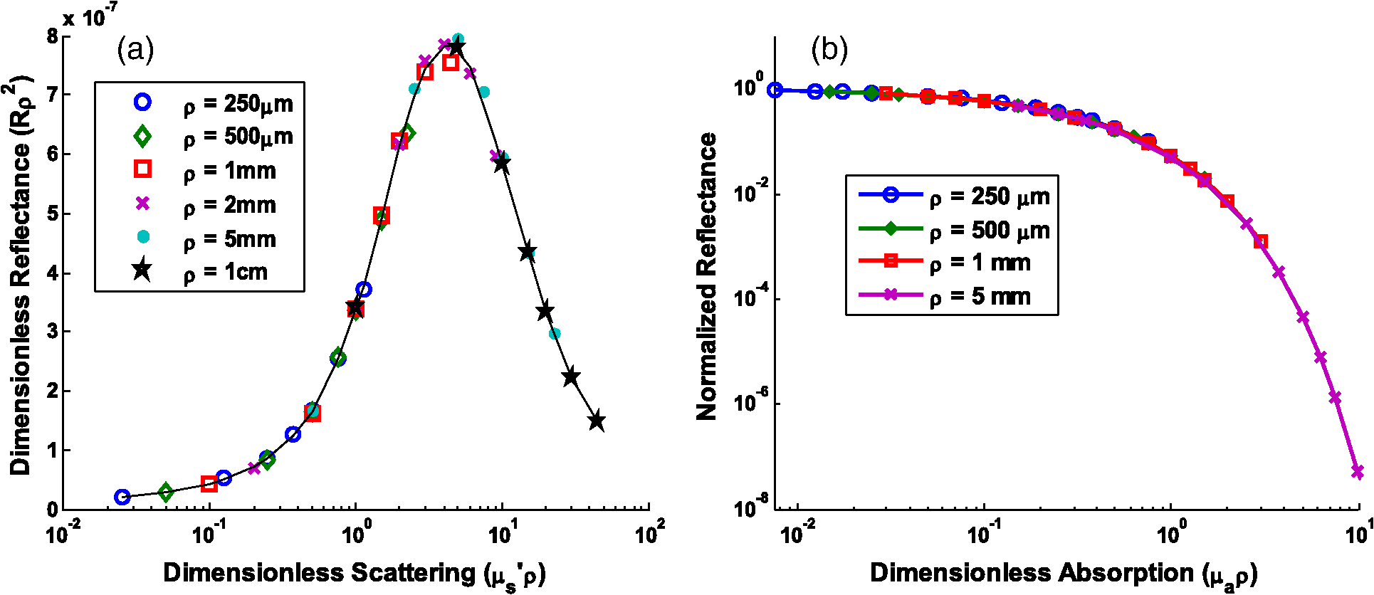 The results presented in Fig. 8 also enable several important observations about reflectance relationships, illustrating the significant variations in reflectance over large dimensionless scattering and absorption ranges, especially for the reflectance versus scattering curve. In contrast to the nearly linear relation of relative reflectance versus scattering illustrated in Figs. 4 and 5, the plot in Fig. 8(a) demonstrates considerable nonlinearity. For low dimensionless scattering, the dimensionless reflectance increases as both scattering and source detector separation increase. But at a given distance, dimensionless reflectance reverses its relationship with and begins to decrease as increases. The observation of this scattering-dependent reflectance relationship is a key component of the generalized reflectance formalism. Several authors have observed this behavior experimentally and it is also predicted by diffusion theory.25,51,52 Further, Kumar and Schmitt related the curve peak to an ideal distance at which reflectance is only slightly dependent on , which they reported to be between 2 and 5 mm, depending on the range of values of interest.51 For a typical tissue value of of , this range of separation distances corresponds to dimensionless scattering values between 2 and 5, which correlates well with the peak of the dimensionless reflectance versus dimensionless scattering curve. It is at this peak value that moderate changes in will result in only minimal change in reflectance, suggesting that reflectance is insensitive to at source detector separations between 2 and 5 mm. A novel and significant observation results from extending this analysis to consider variations in phase function. Figure 9 illustrates the dimensionless reflectance versus dimensionless scattering relationships for a range of phase function values (1.2, 1.75, and 2.3). The critical observation in this figure is the existence of an isosbestic point, where reflectance is not dependent on at a dimensionless scattering value of . (Note that we adopt the term “isosbestic” loosely, with the intent of describing a condition for which one measurement parameter is independent of another.) While reflectance is known to be insensitive to phase function in the diffusion regime (), it is an unexpected revelation that there is an additional singular dimensionless scattering distance, well below the diffusion regime, at which this insensitivity to phase function also exists. Because this isosbestic point is part of the generalized reflectance model, it is applicable to any turbid medium (i.e., independent of tissue model), and is not dependent on the fiber probe (including fiber separation, which is inherently part of dimensionless scattering). Fig. 9Dimensionless reflectance versus dimensionless scattering for a range of phase function values, plus diffusion theory. The three curves with varying values all intersect at a value of 0.7, although diffusion theory does not.  For low dimensionless scattering values, a high corresponds to lower reflectance, as was observed in Figs. 4 and 5 (where ranged from 0.125 to 0.75). As dimensionless scattering increases, however, a point is reached at which reflectance is insensitive to the value of . And at yet larger dimensionless scattering values, a larger value of results in a larger reflectance. As noted earlier, we hypothesize that this is because, in tissues with low , photons with more backward scattering and less forward scattering are more likely to remain close to the source. With high , more forward scattering and fewer backscattering events allow a photon to travel farther from the source before experiencing the high-angle scattering event that will direct it back toward the surface for collection. At large scattering and source-detector separations, this means that the proportion of photons collected at larger source-detector separations to photons collected at smaller separations is higher for large , leading to higher reflectance. For comparison, the diffusion theory equation was used to calculate dimensionless reflectance as a function of dimensionless scattering, and is also included in Fig. 9 (dashed line). Recalling that diffusion theory is not dependent on phase function, above the isosbestic point the diffusion theory plot best approximates the curve, and below the isosbestic point diffusion theory best approximates the curve. This same relationship between diffusion theory and Monte ○Carlo simulations with different anisotropy values was recently observed by Kim et al. for values of and corresponding to dimensionless scattering from 0 to 1,52 which is consistent with our findings. At large dimensionless scattering values, the similarity between diffusion theory and the plot is consistent with the fact that diffusion theory is descriptive of isotropic scattering; since the value corresponds to , the low curve (in this range) is closest to the isotropic case ( and ). We now plot normalized reflectance versus dimensionless scattering, which provides different observations compared with the previously illustrated dimensionless reflectance versus dimensionless scattering relationships in Figs. 8 and 9. Figure 10(a) presents the relationships over a large range of dimensionless absorption values from 0 to 10, and for five values of dimensionless scattering between 0.1 and 8.0. We note that as dimensionless scattering increases, the plots relating normalized reflectance and dimensionless absorption do not monotonically progress. For values of dimensionless scattering below , normalized reflectance is larger for larger values of , as was seen in the relationships illustrated in Figs. 4 and 5. However, for dimensionless scattering values , normalized reflectance is smaller for larger values of . To better visualize this nonmonotonic relation, Fig. 10(b) plots normalized reflectance as a function of dimensionless scattering for a single value of dimensionless absorption, . Fig. 10(a) Normalized reflectance versus dimensionless absorption for five dimensionless scattering values between 0.1 and 8.0. (b) Normalized reflectance versus dimensionless scattering for a constant value of dimensionless absorption of 4.0. 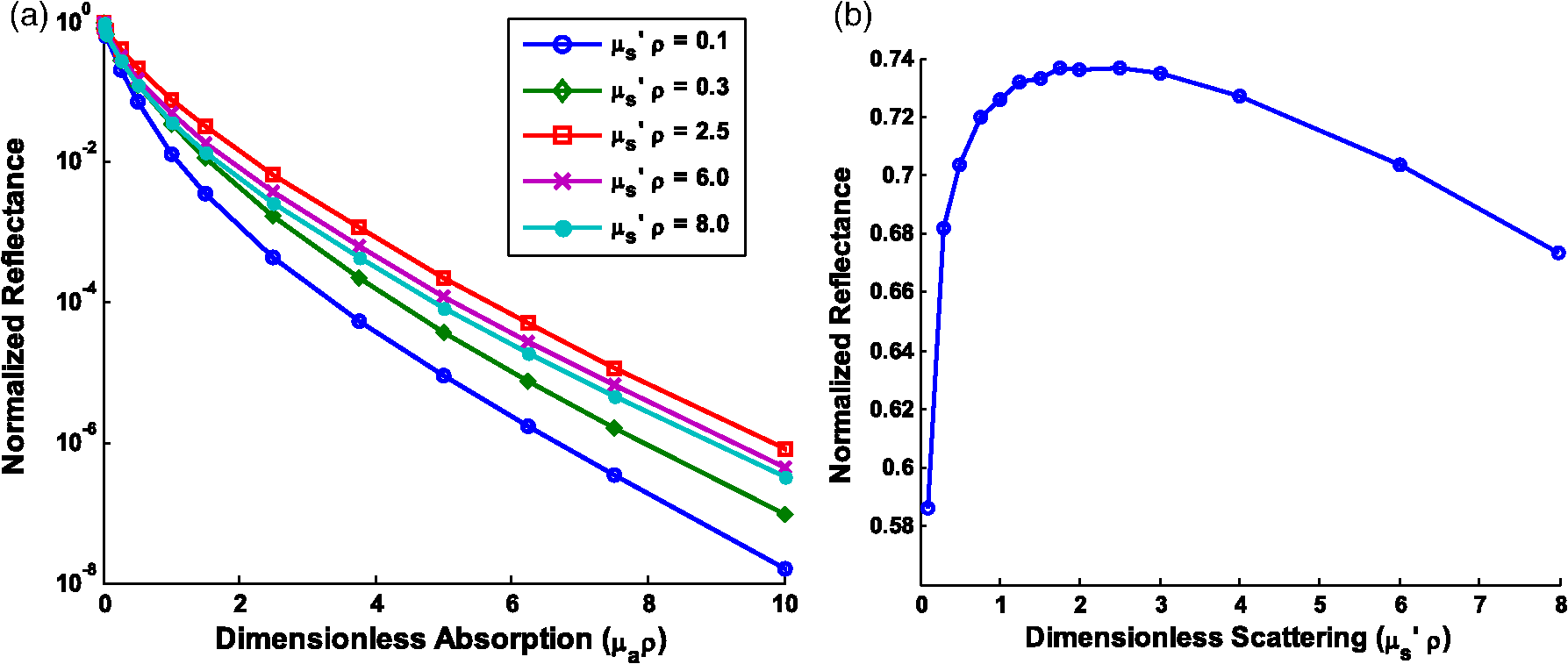 This relationship was explored by Mourant et al., who reported on an optimized source-detector separation for minimizing the effects of scattering.53 In contrast to the analysis of Kumar and Schmitt,51 who identified a source-detector separation that reduced variance in reflectance, Mourant et al. examined the source-detector separation at which variation in photon path length is minimized (enabling application of Beer’s law for determining the absorption coefficient), which they experimentally determined to be . That observation is supported by the results presented in Fig. 10(b), which illustrates that for dimensionless scattering values between and 3, the variation in normalized reflectance (which is directly related to path length) is minimal. When considering average values of in tissue, this range of dimensionless scattering values is consistent with the reported 1.7 mm source-detector separation distance for which normalized reflectance is independent of scattering (at a given ). Like the dimensionless reflectance versus dimensionless scattering relationships, the normalized reflectance versus dimensionless absorption relationships are also dependent on phase function. Figure 11 presents the percent difference between normalized reflectance values with a phase function value .2 and normalized reflectance values with a phase function value . The percent difference is illustrated for a range of dimensionless scattering values between 0.1 and 8.0. As expected, when absorption is zero, the error in normalized reflectance is zero, since, by definition, normalized reflectance is equal to 1.0 when . When dimensionless scattering is low (corresponding to low and/or ), the error in normalized reflectance due to phase function is maximal, reaching as much as 110%. As dimensionless scattering increases and approaches the diffuse regime, the error in reflectance due to phase function variation reduces significantly. However, even at a dimensionless scattering value of 8.0, the maximal reflectance error due to phase function is still over 20%, which is consistent with the known breakdown of the diffusion approximation for large values of absorption. The importance of this observation is that the phase function is an important variable for reflectance even at relatively large source-detector separations. Fig. 11Percent difference in normalized reflectance values between simulations when the phase function parameter and . Percent differences are illustrated for a range of dimensionless scattering values between 0.1 and 8.0.  4.2.1.Error analysis at larger source-detector separationsIn Sec. 4.1.1, the errors in physiological and optical fitting parameters that result from inaccurate assumptions about the phase function were examined for a probe geometry with . Here, we analyze the errors that result from inaccurate phase function assumptions for larger distances: , 1 mm, 2 mm, 5 mm, and 1 cm. The same analysis procedure that was described in Sec. 3.2 and implemented in Sec. 4.1.1 is used here. The errors for all tested reflectance spectra are presented in Table 3, representing the expected errors due to incorrect assumption about the average value of . Errors are smallest for due to the minimal differences in the reflectance versus optical coefficient relationships as a function of phase function at this distance, and are largest (specifically for ) when since the dependence of phase function is greatest at small source-detector separations. However, errors do not decrease monotonically as source-detector separation increases. Rather, for , the error initially decreases when before increasing to a local maximum when and decreasing thereafter as increases to 1 cm. The local error minimum at is the result of the isosbestic point in the reflectance versus dimensionless scattering relationships, because variations in reflectance due to are at a minimum [Fig. 8(a)]. At , the reflectance isosbestic point falls directly in the middle of the physiologically relevant range of for tissue (). With minimal variation in reflectance due to at this point, the inverse modeling errors that result from uncertainty in the tissue phase function are also at a minimum. This indicates that if the phase function of a tissue cannot be accurately estimated (as is typically the case), yet practical constraints do not permit large source-detector separations to take advantage of diffusion theory, it is advantageous to design a probe geometry with a source-detector separation close to 500 μm as a means to minimize errors due to phase function uncertainty. Table 3Average errors resulting from inaccurate assumptions about the phase function of tissue when performing inverse calculations due to incorrect average value of γ used. Reported as averages over all test cases of γ wavelength dependence, and μs′ and μa test spectra.
4.3.Extracting Phase Function InformationWhile extracting and values from tissue has generally been of primary interest, the variation in reflectance as a function of presents an encouraging opportunity to extract additional information about the tissue using DRS. Given that relates to the relative backscattering contributions of a tissue phase function, which is dictated by the size distribution of scatterers, the ability to quantify can provide knowledge about the tissue microstructure. A handful of other authors have also examined this opportunity3,13,54,55 for other measurement geometries (e.g., single-fiber probes that both illuminate and collect light) and have observed that there is not enough information in a single reflectance spectrum to uniquely identify , , and phase function information simultaneously, and therefore, multiple measurements are necessary. In particular, Kanick et.al. have demonstrated that the value of can be extracted from multiple reflectance measurements using multiple single-fiber probes of different diameters.35 Extending this to the two-fiber collection geometry, collecting measurements at various source-detector separations is a natural choice, especially since the reflectance relationships vary significantly as a function of . The implementation of this approach involves measuring reflectance spectra at multiple distances and simultaneously fitting the multiple reflectance spectra to a reflectance model in two dimensions, with both and being independent variables. In addition to the original inverse fitting coefficients described in Sec. 2.1.2, then becomes the sixth fitting coefficient. The reflectance model to which the data are fit is a set of three-dimensional lookup tables for which relative reflectance is defined as a function of , , and . Each three-dimensional lookup table is unique to a single source-detector separation geometry. Experimental reflectance spectra are fit to their respective probe geometry reflectance lookup tables, as would be done with only one reflectance measurement being analyzed, but a least-squares algorithm performs iterative calculations on all data simultaneously, optimizing the physiological fitting coefficients, including , for the entire set of data. Using the and spectra described in Sec. 3.2, reflectance spectra were constructed for a sample value of and for a number of different source-detector separations. Various pairs of reflectance spectra, representing different pairs of source-detector separations, were then analyzed in the inverse direction using the above lookup table approach. In all cases, the extracted optical coefficient values, including the value of , were accurately retrieved with errors . This indicates that with only two separate reflectance spectra and with the differences in source-detector separations as small as 250 μm (when the two reflectance spectra are measured using and 500 μm), not only can errors in the extracted optical properties due to uncertainty in phase function be significantly reduced, but an additional optical parameter can be gained (that of the phase function parameter gamma, ), which can serve to better characterize and differentiate tissue types. 5.ConclusionsThe work reported here constitutes a broad and critical examination of the combined effects of phase function and source-detector separation on the development of diffuse reflectance models for the purpose of extracting estimates about the optical and physiological properties of small volumes of tissue. We have reviewed previous advancements in the understanding of phase function and source-detector separation reflectance relationships, while also contributing a number of novel observations which are combined into a single and comprehensive formalism. Unlike previous developments for diffuse reflectance modeling (for which results were presented in forms specific to a given model construct), this formalism provides a generalized understanding of the ways that measured reflectance can be affected by a wide range of conditions. The key insights of this formalism are as follows:
The novel observations and contributions to this formalism presented in this work include the following:
The presentation of this generalized reflectance formalism is not intended to provide numerical model constructs that can be used directly in experimental diffuse reflectance studies. Rather, our intent has been to provide an intuitive understanding of the trends that form the foundations of useful reflectance models. According to the specific needs of an application, probe geometries should be designed to limit the errors associated with factors such as phase function; reflectance values should be collected as a function of , , and (ideally using Monte Carlo simulations such that input parameters can be most accurately controlled), and those data should be used to construct a probe-specific reflectance model that can be used in the inverse direction to extract accurate tissue optical and physiological properties. AcknowledgmentsThis work was supported in part by the NIN/NCI (U54 CA104677), the Boston University Photonics Center, the NSF Graduate Research Fellowship, and the Center for Integration of Medicine and Innovative Technology (CIMIT). ReferencesJ. Q. Brownet al.,
“Advances in quantitative UV-visible spectroscopy for clinical and pre-clinical application in cancer,”
Curr. Opin. Biotechnol., 20
(1), 119
–131
(2009). http://dx.doi.org/10.1016/j.copbio.2009.02.004 CUOBE3 0958-1669 Google Scholar
I. J. BigioJ. R. Mourant,
“Ultraviolet and visible spectroscopies for tissue diagnostics: fluorescence spectroscopy and elastic-scattering spectroscopy,”
Phys. Med. Biol., 42
(5), 803
–814
(1997). http://dx.doi.org/10.1088/0031-9155/42/5/005 PHMBA7 0031-9155 Google Scholar
F. Bevilacquaet al.,
“In vivo local determination of tissue optical properties: applications to human brain,”
Appl. Opt., 38
(22), 4939
–4950
(1999). http://dx.doi.org/10.1364/AO.38.004939 APOPAI 0003-6935 Google Scholar
C. R. Weberet al.,
“Model-based analysis of reflectance and fluorescence spectra for in vivo detection of cervical dysplasia and cancer,”
J. Biomed. Opt., 13
(6), 064016
(2008). http://dx.doi.org/10.1117/1.3013307 JBOPFO 1083-3668 Google Scholar
E. Salomatinaet al.,
“Optical properties of normal and cancerous human skin in the visible and near-infrared spectral range,”
J. Biomed. Opt., 11
(6), 064026
(2006). http://dx.doi.org/10.1117/1.2398928 JBOPFO 1083-3668 Google Scholar
E. Rodriguez-Diazet al.,
“Spectral classifier design with ensemble classifiers and misclassification-rejection: application to elastic-scattering spectroscopy for detection of colonic neoplasia.,”
J. Biomed. Opt., 16
(6), 067009
(2011). http://dx.doi.org/10.1117/1.3592488 JBOPFO 1083-3668 Google Scholar
G. M. Palmeret al.,
“Monte Carlo-based inverse model for calculating tissue optical properties. Part II: application to breast cancer diagnosis,”
Appl. Opt., 45
(5), 1072
–1078
(2006). http://dx.doi.org/10.1364/AO.45.001072 APOPAI 0003-6935 Google Scholar
I. Georgakoudiet al.,
“Fluorescence, reflectance, and light-scattering spectroscopy for evaluating dysplasia in patients with Barrett’s esophagus,”
Gastroenterology, 120
(7), 1620
–1629
(2001). http://dx.doi.org/10.1053/gast.2001.24842 GASTAB 0016-5085 Google Scholar
R. H. Wilsonet al.,
“Optical spectroscopy detects histological hallmarks of pancreatic cancer,”
Opt. Express, 17
(20), 17502
–17516
(2009). http://dx.doi.org/10.1364/OE.17.017502 OPEXFF 1094-4087 Google Scholar
R. A. Schwarzet al.,
“Autofluorescence and diffuse reflectance spectroscopy of oral epithelial tissue using a depth-sensitive fiber-optic probe,”
Appl. Opt., 47
(6), 825
–834
(2008). http://dx.doi.org/10.1364/AO.47.000825 APOPAI 0003-6935 Google Scholar
A. KienleM. S. Patterson,
“Improved solutions of the steady-state and the time-resolved diffusion equations for reflectance from a semi-infinite turbid medium,”
J. Opt. Soc. Am. A, 14
(1), 246
–254
(1997). http://dx.doi.org/10.1364/JOSAA.14.000246 JOAOD6 0740-3232 Google Scholar
G. Zonioset al.,
“Diffuse reflectance spectroscopy of human adenomatous colon polyps in vivo,”
Appl. Opt., 38
(31), 6628
–6637
(1999). http://dx.doi.org/10.1364/AO.38.006628 APOPAI 0003-6935 Google Scholar
C. K. Hayakawaet al.,
“Use of the delta-P1 approximation for recovery of optical absorption, scattering, and asymmetry coefficients in turbid media,”
Appl. Opt., 43
(24), 4677
–4684
(2004). http://dx.doi.org/10.1364/AO.43.004677 APOPAI 0003-6935 Google Scholar
J. Sunet al.,
“Influence of fiber optic probe geometry on the applicability of inverse models of tissue reflectance spectroscopy: computational models and experimental measurements,”
Appl. Opt., 45
(31), 8152
–8162
(2006). http://dx.doi.org/10.1364/AO.45.008152 APOPAI 0003-6935 Google Scholar
J. C. FinlayT. H. Foster,
“Hemoglobin oxygen saturations in phantoms and in vivo from measurements of steady-state diffuse reflectance at a single, short source-detector separation,”
Med. Phys., 31
(7), 1949
–1959
(2004). http://dx.doi.org/10.1118/1.1760188 MPHYA6 0094-2405 Google Scholar
E. L. HullT. H. Foster,
“Steady-state reflectance spectroscopy in the P3 approximation,”
J. Opt. Soc. Ame. A, 18
(3), 584
–599
(2001). http://dx.doi.org/10.1364/JOSAA.18.000584 JOAOD6 1084-7529 Google Scholar
G. ZoniosA. Dimou,
“Modeling diffuse reflectance from semi-infinite turbid media: application to the study of skin optical properties,”
Opt. Express, 14
(19), 8661
–8674
(2006). http://dx.doi.org/10.1364/OE.14.008661 OPEXFF 1094-4087 Google Scholar
M. Johnset al.,
“Determination of reduced scattering coefficient of biological tissue from a needle-like probe,”
Opt. Express, 13
(13), 4828
–4842
(2005). http://dx.doi.org/10.1364/OPEX.13.004828 OPEXFF 1094-4087 Google Scholar
F. BevilacquaC. Depeursinge,
“Monte Carlo study of diffuse reflectance at source–detector separations close to one transport mean free path,”
J. Opt. Soc. Am. A, 16
(12), 2935
–2945
(1999). http://dx.doi.org/10.1364/JOSAA.16.002935 JOAOD6 0740-3232 Google Scholar
A. AmelinkH. J. Sterenborg,
“Measurement of the local optical properties of turbid media by differential path-length spectroscopy,”
Appl. Opt., 43
(15), 3048
–3054
(2004). http://dx.doi.org/10.1364/AO.43.003048 APOPAI 0003-6935 Google Scholar
S. C. Kanicket al.,
“Measurement of the reduced scattering coefficient of turbid media using single fiber reflectance spectroscopy: fiber diameter and phase function dependence,”
Biomed. Opt. Express, 2
(6), 1687
–1702
(2011). http://dx.doi.org/10.1364/BOE.2.001687 BOEICL 2156-7085 Google Scholar
R. ReifO. A’AmarI. J. Bigio,
“Analytical model of light reflectance for extraction of the optical properties in small volumes of turbid media,”
Appl. Opt., 46
(29), 7317
–7328
(2007). http://dx.doi.org/10.1364/AO.46.007317 APOPAI 0003-6935 Google Scholar
P. R. Bargoet al.,
“In vivo determination of optical properties of normal and tumor tissue with white light reflectance and an empirical light transport model during endoscopy,”
J. Biomed. Opt., 10
(3), 034018
(2005). http://dx.doi.org/10.1117/1.1921907 JBOPFO 1083-3668 Google Scholar
G. M. PalmerN. Ramanujam,
“Monte Carlo-based inverse model for calculating tissue optical properties. Part I: theory and validation on synthetic phantoms,”
Appl. Opt., 45
(5), 1062
–1071
(2006). http://dx.doi.org/10.1364/AO.45.001062 APOPAI 0003-6935 Google Scholar
S. C. Kanicket al.,
“Scattering phase function spectrum makes reflectance spectrum measured from Intralipid phantoms and tissue sensitive to the device detection geometry,”
Opt. Express, 3
(5), 1086
–1100
(2012). http://dx.doi.org/10.1364/BOE.3.001086 OPEXFF 1094-4087 Google Scholar
E. Vitkinet al.,
“Photon diffusion near the point-of-entry in anisotropically scattering turbid media,”
Nat. Commun., 2
(587), 1
–8
(2011). http://dx.doi.org/10.1038/ncomms1599 NCAOBW 2041-1723 Google Scholar
N. RajaramT. H. NguyenJ. W. Tunnell,
“Lookup table–based inverse model for determining optical properties of turbid media,”
J. Biomed. Opt., 13
(5), 050501
(2008). http://dx.doi.org/10.1117/1.2981797 JBOPFO 1083-3668 Google Scholar
S. C. KanickH. J. C. M. SterenborgA. Amelink,
“Empirical model description of photon path length for differential path length spectroscopy: combined effect of scattering and absorption,”
J. Biomed. Opt., 13
(6), 064042
(2008). http://dx.doi.org/10.1117/1.3050424 JBOPFO 1083-3668 Google Scholar
A. TalsmaB. ChanceR. Graaff,
“Corrections for inhomogeneities in biological tissue caused by blood vessels,”
J. Opt. Soc. Am. A, 18
(4), 932
–939
(2001). http://dx.doi.org/10.1364/JOSAA.18.000932 JOAOD6 0740-3232 Google Scholar
L. O. Svaasandet al.,
“Therapeutic response during pulsed laser treatment of port-wine stains: dependence on vessel diameter and depth in dermis,”
Laser Med. Sci., 10
(4), 235
–243
(1995). http://dx.doi.org/10.1007/BF02133615 LMSCEZ 1435-604X Google Scholar
W. F. CheongS. A. PrahlA. J. Welch,
“A review of the optical properties of biological tissues,”
IEEE J. Quantum Electron., 26
(12), 2166
–2185
(1990). http://dx.doi.org/10.1109/3.64354 IEJQA7 0018-9197 Google Scholar
R. Graaff,
“Similarity relations for anisotropic scattering in absorbing media,”
Opt. Eng., 32
(2), 244
(1993). http://dx.doi.org/10.1117/12.60735 OPEGAR 0091-3286 Google Scholar
A. KienleF. K. ForsterR. Hibst,
“Influence of the phase function on determination of the optical properties of biological tissue by spatially resolved reflectance,”
Opt. Lett., 26
(20), 1571
–1573
(2001). http://dx.doi.org/10.1364/OL.26.001571 OPLEDP 0146-9592 Google Scholar
J. R. Mourantet al.,
“Influence of the scattering phase function on light transport measurements in turbid media performed with small source–detector separations,”
Opt. Lett., 21
(7), 546
–548
(1996). http://dx.doi.org/10.1364/OL.21.000546 OPLEDP 0146-9592 Google Scholar
S. C. Kanicket al.,
“Method to quantitatively estimate wavelength-dependent scattering properties from multidiameter single fiber reflectance spectra measured in a turbid medium,”
Opt. Lett., 36
(15), 2997
–2999
(2011). http://dx.doi.org/10.1364/OL.36.002997 OPLEDP 0146-9592 Google Scholar
A. DunnR. Richards-Kortum,
“Three-dimensional computation of light scattering from cells,”
IEEE J. Sel. Topics Quantum Electron., 2
(4), 898
–905
(1996). http://dx.doi.org/10.1109/2944.577313 IJSQEN 1077-260X Google Scholar
L. G. HenyeyJ. L. Greenstein,
“Diffuse radiation in the galaxy,”
Astrophys. J., 93 70
–83
(1941). http://dx.doi.org/10.1086/144246 ASJOAB 0004-637X Google Scholar
J. R. Mourantet al.,
“Mechanisms of light scattering from biological cells relevant to noninvasive optical-tissue diagnostics,”
Appl. Opt., 37
(16), 3586
–3593
(1998). http://dx.doi.org/10.1364/AO.37.003586 APOPAI 0003-6935 Google Scholar
M. CanpolatJ. R. Mourant,
“High-angle scattering events strongly affect light collection in clinically relevant measurement geometries for light transport through tissue,”
Phys. Med. Biol., 45
(5), 1127
–1140
(2000). http://dx.doi.org/10.1088/0031-9155/45/5/304 PHMBA7 0031-9155 Google Scholar
R. K. Wang,
“Modelling optical properties of soft tissue by fractal distribution of scatterers,”
J. Mod. Opt., 47
(1), 103
–120
(2000). http://dx.doi.org/10.1080/09500340008231409 JMOPEW 0950-0340 Google Scholar
S. K. SharmaS. Banerjee,
“Volume concentration and size dependence of diffuse reflectance in a fractal soft tissue model,”
Med. Phys., 32
(6), 1767
–1774
(2005). http://dx.doi.org/10.1118/1.1925807 MPHYA6 0094-2405 Google Scholar
J. M. SchmittG. Kumar,
“Optical scattering properties of soft tissue: a discrete particle model,”
Appl. Opt., 37
(13), 2788
–2797
(1998). http://dx.doi.org/10.1364/AO.37.002788 APOPAI 0003-6935 Google Scholar
B. Gelebartet al.,
“Phase function simulation in tissue phantoms: a fractal approach,”
Pure Appl. Opt., 5
(4), 377
–388
(1996). http://dx.doi.org/10.1088/0963-9659/5/4/005 PAOAE3 0963-9659 Google Scholar
S. K. SharmaS. Banerjee,
“Role of approximate phase functions in Monte Carlo simulation of light propagation in tissues,”
J. Opt. A: Pure Appl. Opt., 5
(3), 294
–302
(2003). http://dx.doi.org/10.1088/1464-4258/5/3/324 JOAOF8 1464-4258 Google Scholar
C. F. BohrenD. R. Huffman, Absorption and Scattering of Light by Small Particles, John Wiley & Sons Inc., New York
(1983). Google Scholar
T. Binzoniet al.,
“The use of the Henyey–Greenstein phase function in Monte Carlo simulations in biomedical optics,”
Phys. Med. Biol., 51
(17), N313
–N322
(2006). http://dx.doi.org/10.1088/0031-9155/51/17/N04 PHMBA7 0031-9155 Google Scholar
T. Binzoniet al.,
“Comment on ‘the use of the Henyey-Greenstein phase function in Monte Carlo simulations in biomedical optics’,”
Phys. Med. Biol., 51
(22), L39
–41
(2006). http://dx.doi.org/10.1088/0031-9155/51/22/L01 PHMBA7 0031-9155 Google Scholar
L. WangS. L. JacquesL. Zheng,
“MCML—Monte Carlo modeling of light transport in multi-layered tissues,”
Comput. Methods Programs Biomed., 47
(2), 131
–146
(1995). http://dx.doi.org/10.1016/0169-2607(95)01640-F CMPBEK 0169-2607 Google Scholar
E. AlerstamT. SvenssonS. Andersson-Engels,
“Parallel computing with graphics processing units for high-speed Monte Carlo simulation of photon migration,”
J. Biomed. Opt., 13
(6), 060504
(2008). http://dx.doi.org/10.1117/1.3041496 JBOPFO 1083-3668 Google Scholar
K. W. Calabro,
“Improved mathematical and computational tools for modeling photon propagation in tissue,”
Boston University,
(2013). Google Scholar
G. KumarJ. M. Schmitt,
“Optimal probe geometry for near-infrared spectroscopy of biological tissue,”
Appl. Opt., 36
(10), 2286
–2293
(1997). http://dx.doi.org/10.1364/AO.36.002286 APOPAI 0003-6935 Google Scholar
A. Kimet al.,
“A fiberoptic reflectance probe with multiple source-collector separations to increase the dynamic range of derived tissue optical absorption and scattering coefficients,”
Opt. Express, 18
(6), 5580
–5594
(2010). http://dx.doi.org/10.1364/OE.18.005580 OPEXFF 1094-4087 Google Scholar
J. R. Mourantet al.,
“Measuring absorption coefficients in small volumes of highly scattering media: source-detector separations for which path lengths do not depend on scattering properties,”
Appl. Opt., 36
(22), 5655
–5661
(1997). http://dx.doi.org/10.1364/AO.36.005655 APOPAI 0003-6935 Google Scholar
U. A. Gammet al.,
“Measurement of tissue scattering properties using multi-diameter single fiber reflectance spectroscopy: in silico sensitivity analysis,”
Biomed. Opt. Express, 2
(11), 3150
–3166
(2011). http://dx.doi.org/10.1364/BOE.2.003150 OPEXFF 1094-4087 Google Scholar
P. Thueleret al.,
“In vivo endoscopic tissue diagnostics based on spectroscopic absorption, scattering, and phase function properties,”
J. Biomed. Opt., 8
(3), 495
–503
(2003). http://dx.doi.org/10.1117/1.1578494 JBOPFO 1083-3668 Google Scholar
BiographyKatherine W. Calabro received her PhD in biomedical engineering from Boston University in 2013. She is currently an R&D engineer at Synopsys, working as a developer on the optical simulation software, LightTools. Irving J. Bigio received his PhD in physics from the University of Michigan in 1974. From then until 2000, he was a scientific staff member at Los Alamos National Laboratory, including leadership of the Laser Science and Applications Group (1988 to 1994). Since 2001, he has been a professor at Boston University, with appointments in biomedical engineering, electrical and computer engineering, physics, and medicine (gastroenterology). He is a fellow of SPIE, OSA, and the American Institute of Medical and Biological Engineering. |
||||||||||||||||||||||||||||||||||||||||||||||||||||||||||||||||||||||||||||||||||||||||||||||||||||||||||||||


