
|
|
1.IntroductionThere is presently a continuing need for bacteria analysis using rapid, portable, reliable, and user-friendly systems.1 The addressed application domains are agro-food safety, clinical microbiology, or the fight against bioterrorism. All these domains would benefit from early detection and identification of microbial contamination or infection in order to undertake as early as possible specific decontamination processes or narrow spectrum antibiotic prescription that will limit the proliferation of drug-resistant antibiotics. Performing analysis on a single bacterial cell rather than on micro- or macrocolonies is a way to drastically increase the rapidity of analysis since it avoids the time-consuming (24 to 48 h) and sometimes not possible cultivation step. Several methods have been developed so far aiming at fast and reliable bacterial identification, e.g., mass spectroscopy, fluorescence immuno-assay, flow cytometry, and polymerase chain reaction. Analysis of microorganisms can also be approached via vibrational methods, i.e., Raman spectroscopy. Raman spectroscopy is an emerging technique in the field of rapid microbial detection and identification.2,3 It enjoys the advantages of being nondestructive and highly specific. For instance, Hamasha et al.4 identified with a good confidence a particular E. coli strain among a set of closely related E. coli strains using spontaneous Raman scattering in conjunction with preprocessing and chemometric techniques. Palchaudhuri et al.5 reported a study about the metabolism of gram-positive and gram-negative. These studies were conducted on colonies and dense pellets. The ability of Raman spectroscopy to probe even a single bacterial cell has been demonstrated: for instance, Huang et al.6 were able to differentiate between growth phases of a single species, and Stöckel et al.7 used surface-enhanced Raman spectroscopy combined with chemometric approaches to identify Bacillus anthracis among 27 strains of Bacillus. Also, spore germination dynamics at the single cell level has been very recently observed8,9 using a novel Raman imaging scheme. Raman spectroscopy studies are traditionally conducted with Raman microscopes. These instruments are usually very versatile and enjoy exquisite sensitivity and signal-to-noise ratio (SNR), but have the disadvantage of being expensive, complex, and bulky. For this reason, one may argue that these systems are poorly suited to routine analysis and, to a lesser extent, to field applications. For instance, Hamasha et al. and Palchaudhuri et al.4,5 used a Jobin-Yvon Horiba TRIAX 550 spectrometer combined with a liquid-nitrogen CCD camera and mounted it on a modified Olympus microscope; Huang et al.6 used a LABRAM 300 confocal Raman microscope (Jobin-Yvon Ltd., Japan). The reasons are first, the need for high spatial and axial resolution ( in volume) due to the minute size of bacteria and, second, the weak intensity of Raman signals (1 photon per 1 million incidents). The former reason explains the use of a confocal microscope, and the latter the use of high-end spectrometers equipped with cooled CCD to enable long acquisition times. Even though laboratory microspectrometers are used, typical acquisition times remain quite long (30 s) for routine analysis. Advanced Raman spectroscopy techniques have been investigated to enhance Raman signals, thus shortening the exposure time to 1 to 6 s: surface-enhanced raman spectroscopy (SERS) allows the use of less complex instrumentation, for instance, the BioParticleExplorer coupled to a TE-cooled HE532 Jobin-Yvon spectrometer.7 However, we preferred not to investigate SERS because the current technology suffers from drawbacks, such as poor reproducibility and the need for particular substrates or sample preparation, which hinder its application to routine biological analysis.2 Our system is the first to combine lensfree imaging with Raman spectroscopy. We found that lensfree imaging is sensitive enough to detect small bacteria aggregates typically composed of less than a dozen individuals. In our system, the lensfree image has a wide field of view (FOV) of . This wide FOV enables us to rapidly locate regions of interest, even in a dilute sample. Once a small group of bacteria has been selected, one may focus the probing laser beam on that area. It was observed that the diffraction pattern from a single individual interacting with the focused beam is sensitive enough to allow precise alignment of the beam with the bacteria. This diffraction pattern may also be used to gain insight on bacteria morphology, complementing the Raman analysis. This scheme avoids the use of a standard microscope, in particular, the use of multiple microscopic objectives of increasing magnification generally required during the alignment step. The idea of multimodal architecture has already been investigated in order to increase the instrument’s overall performances, but results in by far more complex instrumentation.8,10 By contrast, our goal is to use the additional modality to simplify the system and accelerate the operation flow. Our system also integrates a high-throughput virtual slit (HTVS) spectrometer prototype developed by Tornado Spectral Systems (Canada), which combines high throughput in the region of interest (500 to ), acceptable spectral resolution (), middle price, and a very good compactness. The present study focuses on the Raman scattering modality, which is assessed in terms of discrimination and classification of bacteria at the species level. Spectral data obtained from individual bacterial cells are preprocessed and analyzed with a data classification approach, the so-called support vector machine (SVM) technique. A dataset of 1205 Raman spectra obtained from single bacteria of seven different species has been recorded using shorter acquisition time (10 s) than those usually employed in spontaneous Raman spectroscopy (30 s),11 or in the range of SERS (6 s).7 The obtained classification score of 89% demonstrates the ability of our system to perform single bacteria analysis and, more precisely, to identify bacteria at the species level. This study, thus, suggests that reasonable performance on bacteria identification is possible using short acquisition times and an optimized spectrometer. 2.Experimental Section2.1.Lensfree Imaging Sample HolderThe sample, typically a 5-μl droplet containing bacteria, is deposited and left to evaporate for 2 min on a quartz cover slip (TedPella Inc., Redding, California, ) that was placed on an 8-bit CMOS sensor (MT9P031, Aptina Imaging, San José, California). This configuration [illustrated in Fig. 1(b)] implements the lensfree on-chip technique reported in Allier et al.12 Briefly and as illustrated in Fig. 1(a), the image formed in transmission onto the sensor results from the interference between the light coming directly from the illumination source (here a laser beam) and the light scattered by the bacterial cell(s). Fig. 1Lensfree imaging module. (a) Schematic illustrating the principle of lensfree image formation. (b) Picture of the developed module used as the sample holder. 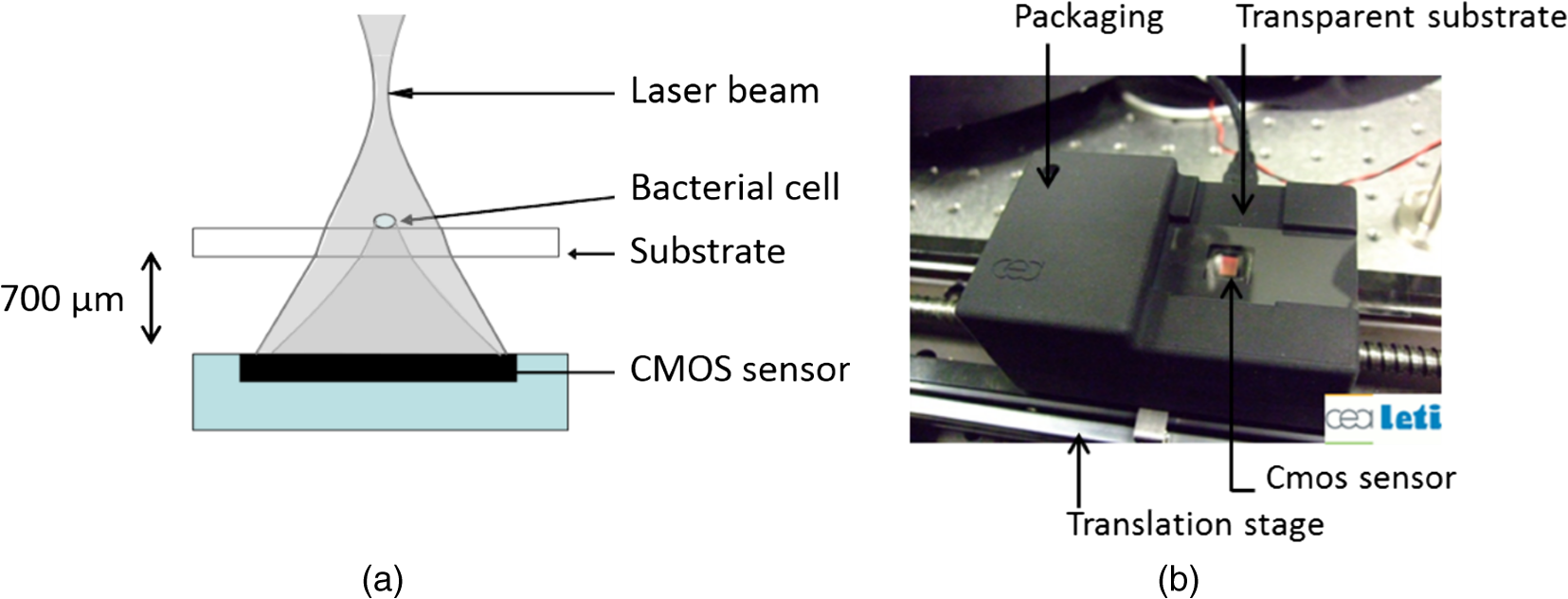 This technique succeeded in monitoring and counting cells, single bacteria, or viruses using a light-emitting diode as the illumination beam and a thin wetting film enabling enhancement of the micron-sized particles by creating microlenses-like liquid films on top of them.12–14 In this study, no wetting film is used since it would be detected by Raman spectroscopy rather than the specific signal arising from the bacteria. Yet, the small aggregates obtained after evaporation are efficiently detected. We routinely detected aggregates composed of as little as 5 to 10 individuals. Depending on the laser spot size impinging the sample, the FOV can be varied from to . More precisely, these large and small FOVs are obtained when the laser spot size is about the sensor size and when it is comparable to the size of the bacterium to probe (1 μm), respectively. In this latter configuration, the image formed onto the CMOS sensor is due to forward elastic scattering only and, thus, reveals both the laser spot and the bacterium patterns (Fig. 2). The operator is then able to accurately monitor the alignment of the probe onto the sample. Fig. 2Lensfree images of single B. cereus illustrating lateral alignment process. On the left, laser probe is correctly aligned onto the bacteria. On the right image, the laser probe is m right misaligned. Central cross marks the position of bacteria.  In sum, the entire droplet as well as a zoomed view of a single bacterium can be easily observed and accurate lateral alignment of the laser probe is possible, thanks to this so-called lensfree (or lensless) based scheme. Moreover, a forward scattering pattern, the so-called lensfree image, can be collected for each probed bacterium in order to extract its morphological characteristics. In practice, the spot size is easily adjusted by translating the sample along the laser beam using a vertical translation stage mounted on the optical bench, and the XY laser probe alignment is achieved using a double translation stage (PI micos VT-75) mounted below the lensfree module, as illustrated in Fig. 3 and described in Strola et al.15,16 Fig. 3(a) Schematic of the integration of lensfree imaging in the Raman optical bench. (b) Illustration of the four-steps operation flow: (1) using a high Z value, thus large spot size, the entire droplet is observed with diffraction patterns corresponding to bacteria; (2) using intermediate Z value enables the operator to choose the bacteria of interest and align in XY the laser probe onto it; (3) using a Z value 70 microns above the Raman focal position, the interference pattern can be collected by the lensfree imaging module; (4) Raman focal position is found when the diffraction pattern blurred due to the laser spot size being smaller than the bacteria.  2.2.SetupFigure 4 shows schematics of the setup [Fig. 4(a) and a picture [Fig. 4(b)] of the lensfree imaging based Raman microspectrometer.12 Fig. 4(a) Schematic of the optical architecture. (b) Picture of the apparatus consisting of (1) 532-nm continuous wave TEM00 laser head, (2) optical density (0.3), (3) razor-edge 45 deg of incidence filter, (4) , microscope objective, (5) lensfree imaging module on which is placed the sample, (6) two notch filters and plane-concave focusing lens, (7) optical fiber 105 μm , (8) Tornado Spectral Systems prototype spectrometer, (9) vertical motorized translation stage, (10) and (11) translation stage in the plane of the optical table, XY.  A 532-nm laser (Spectra Physics Excelsior 532-50-CDRH, Santa Clara, California) is both the Raman excitation light and the alignment light. By contrast, most Raman microscopes integrate separated light sources and paths, thus increasing the complexity and the risk of misalignments. The 50-mW optical output power is reduced by means of an optical density down to few nanowatts during the alignment step and to 34 mW for the Raman spectra collection. A razor-edge filter (Semrock LPD01-532RS-25, Rochester, New York) steers the laser beam at 45 deg into a microscope objective (Olympus LMPLFLN, Japan) that illuminates the sample from above. The magnification combined with the very high laser beam quality () enables a spot size of in diameter at the beam waist together with a good wave front quality, an important specificity for large field lensfree imaging. When the sample is in the beam waist position [Fig. 1(a)], Raman scattered light is generated and collected by the microscope objective, transmitted through the razor-edge filter, filtered from elastic scattering by two notch filters (Semrock NF03-532E), and, finally, focused into the spectrometer optical fiber (Thorlabs M18L01, 0.22 NA, Newton, New Jersey) using a 50-mm achromatic lens. The system, therefore, operates in a confocal configuration, similar to a traditional Raman microscope. The optical fiber tip (105 μm) acts as the pinhole and yields an axial resolution of 2 microns. The spectrometer, APEX-532, is a custom-built unit consisting of the best features from Tornado Spectral Systems’ HyperFlux 532 spectrometer and Ocean Optics QE65000 detector (Hamamatsu, Japan, thermoelectric cooled). The HTVS technology allows this unit to generate both broadband (spectral range from to ) and high-resolution () spectra while enhancing the optical throughput in the wavelength range of interest for bacteria analysis range (500 to ). This patented technology modifies the shape of the beam in the spectrometer with total optical throughput and differs from conventional spectrumeters that use a narrow entrance slit to achieve higher resolution at the cost of throughput. HTVS technology alleviates the classical trade-off between resolution and throughput in a dispersive spectrometer: the light beam is expanded while the total flux is preserved, allowing for an improvement of the performance.17 As an example, Fig. 5 shows two spectra of the same polystyrene sample (1 mm thickness) acquired with a 1-s acquisition time on our platform and on the Horiba (Japan) LabRAM Aramis commercial system, respectively. Acquisition parameters were fixed to compare the two setups. The laser power was set to 34 mW in both systems and the spot size to 1 μm. As a side note, one may observe small lateral shifts originating from the difference in resolution as well as a slightly different calibration of the two instruments. We point out that this discrepancy does not affect later classification performance. We note that our setup performs better in terms of net intensity along the spectral range from 600 to . The SNR varies along the spectra depending on the light throughput curve that is different for the two acquisition systems. We calculated the SNR for the polystyrene peaks at 1001, 1193, and to give a representative idea. Values are summarized in Table 1. Fig. 5In the spectral range from 600 to , the setup used in this study (dotted line) shows a better net intensity and signal-to-noise ratio (SNR) with respect to a classical Raman microspectrometer, in this case Horiba LabRAM Aramis (continuous line). We used 34-mW laser power at the polystyrene sample (1 mm thickness), with a spot size of 1 μm, in both measurements for 1-s acquisition time. 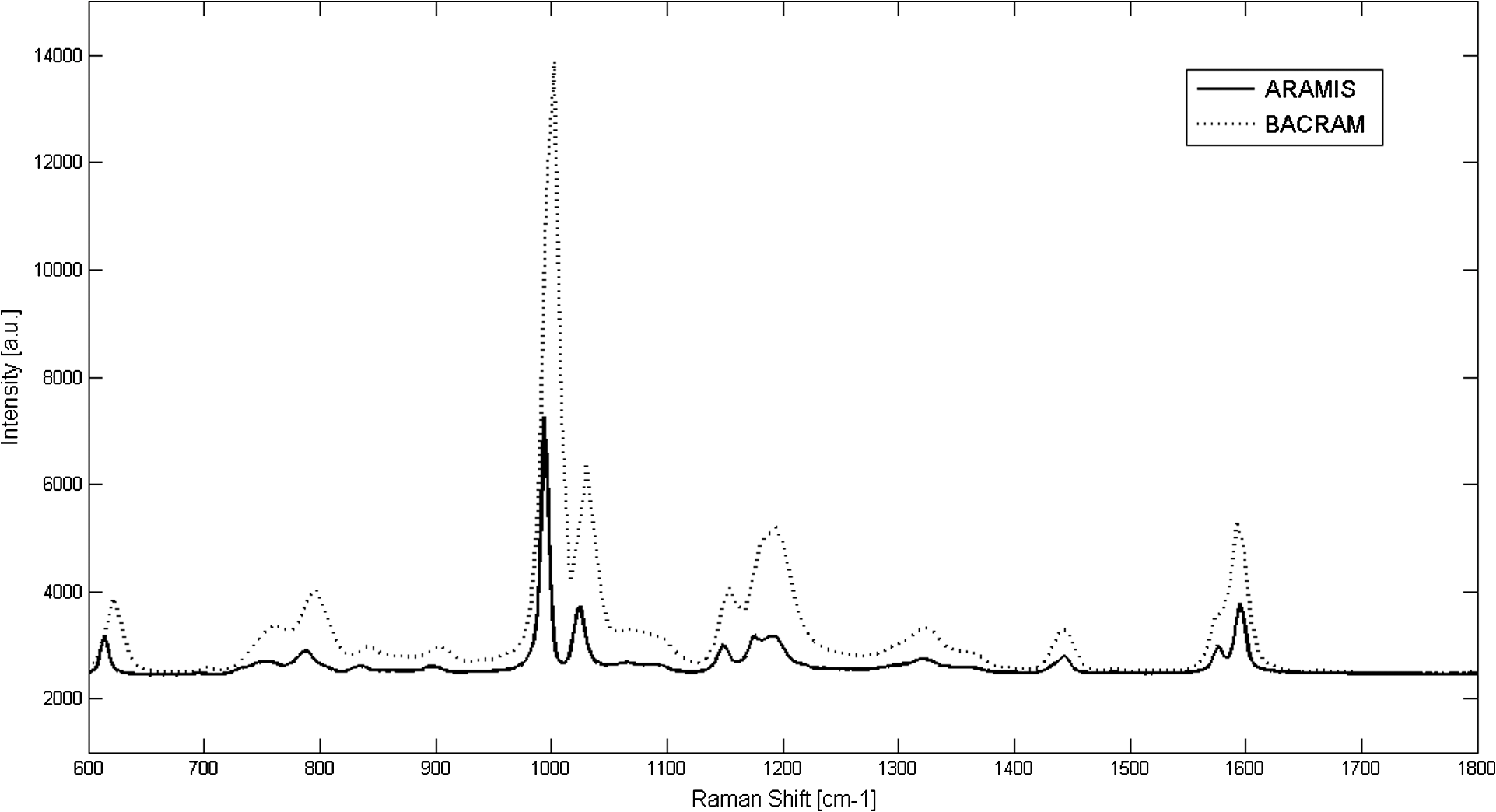 Table 1Signal-to-noise ratio (SNR) values for the different spectrometers compared at selected peaks of polystyrene sample.
APEX-532 has been calibrated with Hg lamp calibration and polystyrene has been used as a daily reference sample. Although the performance in SNR is in favor of the APEX-532 on very Raman-active samples, such as polystyrene, the situation is different for the very weak bacteria signals. Figure 6 shows representative bacteria spectra acquired at 30 s [Fig. 6(a)] and 60 s [Fig. 6(b)] on our instrument and the Aramis, respectively. SNR values are also included. We again note the distinct throughputs of the two instruments. Our instrument enhances the range between 600 and , which results in a lower peak height at compared to the Aramis, which has a flatter response. In terms of SNR, the Aramis performs better at both 30 and 60 s integration. This was expected since, among others, the Aramis uses a detector cooled at compared to for the APEX-532. When increasing the acquisition time from 30 to 60 s, the measured SNR improves from 2.17 to 2.99 for the APEX-532, while it increases from 5.73 to 9.82 for the Aramis system. The lower relative increase in SNR for the APEX is explained by the fact that the instrument was optimized for short acquisition times and weak Raman signals.17 This is also in agreement with our choice of using APEX-532 in this application. The price paid in SNR for decreasing the integration time to 10 s is better offset by the gain in acquisition time with APEX than with Aramis. Fig. 6B. subtilis spectra and SNR values for acquisition time of 30 s (a) and 60 s (b) with our instrument (Bacram, simple line), and with the Aramis setup (in bold), respectively. 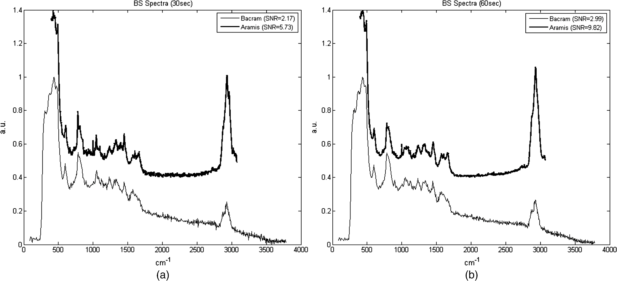 All these optical components, except for the spectrometer unit, are mounted on a single vertical translation stage (PI micos VT-75) with a resolution better than 0.4 μm, which allows an accurate adjustment of the focal position. Its large course (50 mm) also enables the adjustment of the illumination spot size onto the sample according to the lensfree based method previously described. The translation stages, spectrometer, and CMOS sensor are controlled via a program developed under the software Labview® (version 2011). This program is a useful interface that allows full control of the setup. Alignment protocol takes from the moment the droplet has been evaporated until the Raman acquisition starts. The Z position provided by the lensfree based scheme is to 2 μm off the correct Raman focal position, which is found by monitoring the appearance of the C-H band at in the Raman spectra using minute translation steps (0.4 μm). An exposure time of 1 s is sufficient to obtain a Raman signal and guarantees a rapid alignment. Interference pattern collection is very fast, in the millisecond range, and the Raman exposure time has been decreased to 10 s, thanks to the high spectrometer throughput. Typically, it takes 25 min to collect 30 spectra from 30 different single bacteria in a single droplet. Scattering patterns and Raman spectra are analyzed off line using MATLAB® (R2013a) and RStudio programs, respectively. This paper focuses on the Raman scattering analysis (preprocessing and classification techniques) to demonstrate the scheme’s feasibility to collect Raman comprehensive spectra and to identify bacteria. Scattering patterns analysis will be reported in a future paper. Last, a direct imaging path was added to the system for validation purposes. The direct image was used (1) to facilitate system alignment, (2) to confirm that the particles detected in the lensless image were actual bacteria, and (3) to evaluate the detection limit in the lensless image. The detection limit was found to be small bacteria aggregates composed typically of 5 to 10 individuals. Direct imaging was implemented using a mirror in the Raman path. Light from a white illuminator is reflected by the mirror back to a CMOS sensor (Thorlabs, Newton, New Jersey) equipped with a Navitar objective. The magnification of this direct imaging path was set to 40. An illustration of the full optical path is presented in Fig. 4(a). 2.3.Biological Protocol and Sample PreparationMicroorganisms E. coli (ATCC 9637), B. subtilis (ATCC 23857), S. epidermidis (ATCC 14990), B. cereus (ATCC 10702), B. thuringiensis (ATCC 33679), M. luteus (ATCC 4698), and S. marcescens (ATCC 27137) were purchased from American Type Culture Collection (Manassas, Virginia). B. subtilis, B. cereus, B. thuringiensis, M. luteus, and S. marcescens were grown overnight in Trypcase Soja Broth (Fluka 22092) at 30°C for Bacillaceae family and M. luteus and 26°C for S. marcescens. E. coli and S. epidermidis were grown overnight in Luria Broth (Sigma-Aldrich L2542, St. Louis, Missouri) at 37°C. Each strain was cultivated in one broth culture in a liquid medium overnight (16 h). At the end of this culture step, all the bacteria have reached the stationary phase. Bacteria were then washed twice with Milli-Q ultrapure water by centrifugation (3500 rpm for 2 min) in order to ensure the complete removal of the medium. The pellet is then resuspended in 100 μL of Milli-Q water and absorbance measurements were made at (photospectrometer Uvicon923—BioTek Kontron, Winooski, Vermont). A stock solution with an optical density of 1 was then prepared, and Raman experiments were performed with a 1/100 dilution in MilliQ water of the stock solution. The bacteria solution is then immediately processed with Raman acquisition to guarantee the biological homogeneity of the analysis during the stationary growth phase. An amount of 5 μL for each bacteria solution is pipetted on top of a quartz coverslip (TedPella Inc., Redding, California, and 0.5 mm thickness) previously rinsed with ethanol solution at 70% (Sigma-Aldrich, St. Louis, Missouri) and dried with nitrogen. This protocol ensured that all bacteria are in the same growth phase, independent of the strain prior to the Raman measurement. Before starting the measurements, we let the liquid drop containing bacteria evaporate to create an investigation region of a few millimeters in diameter. After each analysis, the quartz coverslip is carefully cleaned in an ultrasonic bath (Novatec, Baltimore, Maryland) for 10 min. For each strain, we collected Raman spectra over 30 different single-cell bacteria at the stationary growth phase. This protocol allows us to minimize the biological variability of the various metabolism steps at the different growth phases. Each Raman acquisition has been performed with an integration time of 10 s. The background signal of the quartz coverslip, to be subtracted from Raman spectra of bacteria during data processing, is acquired at the same integration time at five random surface points before the deposition of the bacteria solution drop. Spectra were cropped to spectral regions of interest (ROIs) ranging from 650 to and 2600 to , which cover the biochemical specific peaks of bacteria.18,19 2.4.Raman Spectra AnalysisData analysis (spectra preprocessing, calculation of indicators, and classification) was performed using the R software environment, with existing functions or routines specifically developed for this use. Preprocessing was applied to prepare the Raman spectra for the classification algorithm. The first step of spectrum preprocessing consists of cosmic spikes removal using the method proposed in Espagnon et al.20 Then, several treatments have been considered for the input data to the classification method. From the simplest to the most complex, we tested the raw spectrum, smoothed and normalized, the first derivative, and the normalized net spectrum after background subtraction. Smoothed signal and first derivative are calculated by Savitzky-Golay polynomials filters21 (degree 4, on 9 points). As the distance between two channels is in the ROI, a filter width of 9 points corresponds to . This is to be compared to a full width at half maximum equal to for the quartz peak at . The aim is to reduce the noise in the signal without peak distortion and loss of intensity. Background subtraction is more complex and includes several steps. The background is composed of signals from the quartz substrate and the sample autofluorescence. For estimating the quartz signal, we consider the mean quartz spectrum, calculated using several quartz spectra acquired on the same coverslip at the same date as the bacterium spectrum. We then fit the mean quartz spectrum to each bacteria spectrum on the large peak spreading from 200 to , specific to quartz [Fig. 7(a)]. An approaching method is presented in Beier et al.,22 with a rather different spectrum topology. Fig. 7Examples of E. coli spectrum: (a) raw spectrum and mean quartz spectrum after fitting on the main peak of quartz (both spectra were smoothed). The high contribution of the quartz in the bacterium spectrum can be observed. (b) Dotted line: spectrum obtained after subtracting the quartz contribution estimated by fitting. Solid line: spectrum after subtraction of quartz contribution and 600 iterations of the Clayton’s algorithm (specific net spectrum).  A constraint on the relative level of quartz signal, which has to be smaller than the bacteria spectrum on the region up to , is added to the fitting procedure. The fitted mean quartz spectrum is then subtracted from the bacteria spectrum. We deal with sample autofluorescence using the Clayton’s algorithm (also used in the sensitive nonlinear iterative peak-clipping algorithm23), applied with a neighborhood window of three channels. This algorithm is iterative: when the number of iterations grows, the calculated background level drops. At the end of the process, the quartz contribution is extremely reduced and the bacteria peaks are, thus, emphasized, which facilitates their study. The resulting spectrum is called specific net spectrum [Fig. 7(b)]. Normalization is the last step before clipping the spectrum to the ROI. It is obtained by dividing the signal by its mean value on a chosen ROI. This enables us to have all spectra at the same scale, independent of factors that may vary between two spectra or two experiments (laser power, etc.). For 100 spectra, preprocessing time is for data transfer and 7 s for cosmic spike removal. Background subtraction time depends on the number of iterations applied. For example, 600 iterations require 5 s, while 2500 require 30 s. These estimates are given for a PC equipped with an Intel Core i5 at 2.40 GHz and 8 GB of RAM. Processed spectra are stored in long-term memory for future reuse. 2.4.1.Indicators of spectra qualityIn order to assess the overall quality of the spectra, we used two indicators: the standard deviation of the means (SDM) and SNR. SDM of a set of spectra is the mean standard deviation of channels normalized to the standard deviation of the mean spectrum.7 We calculate it on the normalized specific net spectra representative of a same strain. Low values of SDM indicate low variability by channel and high reproducibility of the spectra set, while high values, close to 1, are associated with high noise levels or disparities in the spectra set. SNR is a quality indicator of the individual spectra. We define it as the mean of the specific net signal in a region specific to bacteria, here the peak at , divided by the standard deviation of the specific net signal in a region without bacteria signal, here the 2000 to region. For example, the SNR for the spectrum of Fig. 7(b) is 3.7 for the peak at . In addition to these two quantitative indicators, more qualitative tools may be used: the dendrograms measure distances between spectra and represent the latter under a tree according to the distance that separates them. Dendrograms, which are the calculation of the mean spectra plotted for each strain and are associated with principal component analysis, enable us to screen simple outliers and to identify groups of spectra with diverging trends. 2.4.2.Classification methodThe classification algorithm used here is SVM, which is a supervised classifier (function “svm” of the R package “e1071,” interfacing the “LIBSVM” library,24 with a linear kernel). For cross-validation, all species strains were represented in the reference base. One tenth of each strain, for all strains, was randomly chosen and removed from the reference base to form the validation base. Thus, a 10-fold cross-validation enables us to test all spectra. We repeat the process 10 times and output a mean confusion matrix as well as the mean global success rate and standard deviation of the global success rate. We used two scenarios for the cross-validation. In one scenario, one tenth of the spectra comprising the validation base were selected regardless of the acquisition date. Spectra from a same date are allowed to appear in the reference and in the validation base (although a given spectrum cannot be in both simultaneously). In the second scenario, we select the spectra used for validation based on the date. In this setting, spectra from a given strain and date are not allowed to be present in both validation and reference base. This second scenario prevents classification biases due to experimental and preprocessing artifacts. The first scenario is more favorable and, as expected, our success rates were higher. In the second scenario, our results presented higher disparity according to bacteria strain and acquisition date. This point will be detailed at the end of Sec. 4. 3.Results3.1.Raman SpectraFigure 8 shows typical images and spectra captured using our system. A blow-up of the two ROIs is displayed in Fig. 9. Fig. 8Validation of the lensfree ability to probe a single bacterial cell and collect scattering pattern and Raman spectrum. (a) Direct space white light image of the bacterial cell. (b) Backscattered image showing the laser probe is well aligned with the cell. (c) Forward scattered pattern collected using lensfree module. (d) Raman spectrum generated by the bacteria cell.  Fig. 9Mean normalized net spectrum for E. coli and B. subtilis. Dotted lines correspond to three times the mean standard deviation of the mean value, divided by the square root of the number of spectra (154 and 273 for E. coli and B. subtilis, respectively). Raman bands detected are indicated and are found consistent with previous studies.25 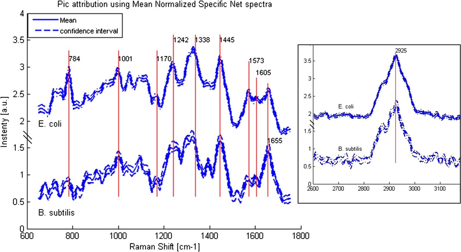 We display the average of processed Raman spectra acquired for B. subtilis and E. coli bacterial strains with a 10-s exposure time. The spectra consist of bands representing the cell contents: proteins, lipids, and nucleic acids. In particular, the peaks centered at 784, 1001, 1170, 1242, 1338, 1445, 1573, 1605, 1655, and are detected for both strains. Typical signatures of cell components are CH stretching vibrations and are visible at . The contribution from various proteins is related to a band centered at . In particular amide I, mainly associated with the stretching vibration and directly related to the backbone conformation, is detected in this band. Amide III, known as a very complex band dependent on the details of the force field, the nature of side chains, and hydrogen bonding, is revealed by the band. DNA bands arise in the region via guanine and adenine nucleobases, but an overlapping with amide II contributions (, N-H, and C-N stretching) can be reported. bending vibrations are assigned to the band at and give contribution from various lipids. Bands arising from amino acid side chains appear at 1605 and : the signals can be both assigned to phenylalanine. Tyrosine and phenylalanine give origin to the signal detected at . The region shows the fingerprint of the cytoplasm fraction detected via DNA vibration. The band centered at is covered by cytosine stretching vibrations as part of the DNA contribution. The peak assignment, based on previous works,15,26 is summarized in Table 2. Table 2Assignment of Raman bands detected.
3.2.Database DescriptionWe conducted an acquisition campaign in order to populate a reference database composed of the seven strains of bacteria described in Sec. 2.3. Spectra were measured for four consecutive days, with 120 spectra per day (four strains of bacteria, 30 spectra each). In addition, spectra from other days were added to the database to reach a final count of 1205. Each spectrum was collected using an integration time of 10 s. SDM and SNR for each strain were calculated (Table 3). SDM values are rather high, from 0.6 for S. epidermidis to values , with 1.3 for E. coli and 1.7 for S. marcescens, mainly due to the low acquisition time. We find the same trend with SNR. Mean SNR ranges from 3 for the noisiest series (S. marcescens and E. coli) to 6 for the best series (M. luteus and S. epidermidis). Table 3Standard deviation of the means (SDM) and SNR values for the different bacteria investigated.
The dendrograms, PCA, and mean spectra, plotted for each strain, brought out some aberrant spectra, probably due to a contamination of the quartz substrate. That may explain the higher value of SDM obtained for M. luteus (0.8), compared to S. epidermidis, although SNR are similar. 3.3.Preprocessing ChoiceIn this section, we investigate the various preprocessing options described above, namely, smoothed spectrum, first derivative, and net spectrum. We also discuss the choice of the ROI and number of Clayton iterations for computing the net spectrum. We use the classification score (calculated by cross-validation) as the figure of merit. We first apply a fully randomized cross-validation (first scenario mentioned in Sec. 2.4.2). Figure 10 shows the classification score obtained with the specific net spectrum as a function of Clayton iterations number and ROI. As expected, the use of two ROIs rather than a single ROI yields better scores. The score plateaus around 84% after 3000 iterations. We, therefore, fix the number of iterations to 4000 for the net spectrum in the sequel. We now compare the performance of the various preprocessing options. For now, the net spectrum is computed using a quartz signal acquired on the same slide on the same date as the data. Results are summarized in Table 4. The first derivative method (74.7% of success) is outperformed by both smoothed spectrum (84.5%) and net spectrum (86.5%), with a slight advantage overall for the net spectrum. Fig. 10Classification rate according to the iteration number in the Clayton’s algorithm, for each region of interest (twofold cross-validation).  Table 4Mean classification rates and standard deviation according to the type of preprocessing (fully randomized 10-fold cross-validation).
Note: ROI, region of interest. Then, we evaluate the preprocessing performance using the date-based cross-validation described in Sec. 2.4.2. Two methods for computing the net spectrum are now considered. First, the subtracted quartz signal was acquired on the same date. Second, the subtracted quartz is the mean of all quartz signals across all experiments. In this setting, we find that the net spectra calculated with the mean quartz and smoothed spectra have comparable performances (79.8% and 80.9% success, respectively, on the Bacillus family) and outperform the net spectra calculated with the quartz signal from the same date (75.9% success). Although these results do not indicate a significant advantage for quartz and background subtraction over a simple smoothing, it is noteworthy that no significant sample autofluorescence was observed in this dataset. The advantage of nonspecific signal subtracting would be more remarkable otherwise. With this in mind, we chose the net spectrum as the preprocessing method for the results presented in this work (with a quartz signal acquired on the same date). 4.Discussion and ConclusionsThe classification performance of our instrument was evaluated using the two cross-validation scenarios described in Sec. 2.4.2. We begin with the first scenario in which a given date is susceptible to appear in both the reference and the validation base. The successful identification rates are presented in the form of a confusion matrix [Fig. 11(a)]. It is interesting to note that the highest success rates () are obtained for M. luteus and S. epidermidis, which present the highest SNR and good SDM. On the contrary, S. marcescens, which has the highest SDM and lowest SNR, obtains a classification rate of only 79.9%. The most frequent confusions are observed between B. cereus and the other Bacilli or between B. cereus and the two Enterobacteriaceae, and between the two Enterobacteriaceae themselves. Fig. 11Mean confusion matrix using 10 s acquisition time and support vector machine classification technique. (a) Species-level classification (). (b) Families-level classification (). 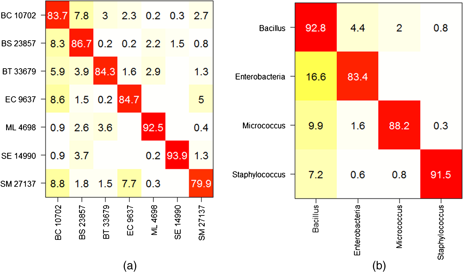 One may also consider the simpler task of identifying bacteria families rather than bacteria strain. The resulting confusion matrix is displayed in Fig. 11(b). A very satisfying classification rate was obtained for the Bacillus family, with only 7.2% of the Bacillus spectra identified as non-Bacillus. The lowest classification rate (83.3%) was obtained for the Enterobacteria. In an attempt to measure the influence of the acquisition time on the spectrum quality and further on the classification results, experiments were carried out on E. coli and S. marcescens with a longer acquisition time, equal to 20 s. The new values of SDM are clearly lower, 0.7 for both strains, respectively. Both E. coli and S. marcescens achieved an SDM value of 0.7, which represents a decrease of 1.9 and 2.7 for E. coli and S. marcescens, respectively. Correspondingly, a net improvement in SNR was observed (5 for E. coli and 6 for S. marcescens corresponding to gains of 1.5 and 1.9, respectively). The new confusion matrix is presented in Fig. 12(a). The classification rates for E. coli and S. marcescens are improved, as they grow, respectively, from 84.7 to 91.1% and from 79.9 to 95.6%. This has a positive influence on some of the other bacteria as well, with the mean success rate increasing to . The same trend is noted on family classification: the success rate is improved by 10% for the Enterobacteriaceae, and by a few percent for the Bacilli [Fig. 12(b)]. As expected, these results suggest that a longer acquisition time improves the classification results. Yet it is interesting to note that 10 s yields very satisfactory results. Fig. 12Mean confusion matrix obtained using longer exposure times (20 s instead of 10 s) for E. coli and S. marcescens. (a) Classification at the strain level (). (b) Classification at the family level ().  We now turn to our second cross-validation scenario mentioned in Sec. 2.4.2. There, a given strain and date is not permitted to appear at the same time in the reference base and in the validation base. In this case, we obtain a lower global success rate. We observe disparities according to strain and acquisition dates. The mean success rate is 84.0% for B. subtilis, which presents the highest number of experiment dates, in the Bacillus family. However, the results are largely dispersed with the highest success rate being 100% and the lowest 45% depending on the date. For S. epidermidis, which is the least represented in the database in terms of experiment dates, the mean identification rate in the Staphylococcus family falls to 55.3%, with results spreading from 21.1 to 86.7% according to the date. The dispersion of these results depending on the date hints at a possible influence of other important factors like growth phase, nutrition, or matrix (sterile or real) effects that would need to be taken into account in the dataset. We have already started to explore this possibility and found, for instance, that our system is able to discriminate between different growth phases of E. coli and B. subtilis.27 Note as well that the mentioned dispersion could be partially attributed to preprocessing the spectra using a quartz signal acquired by date. Nevertheless, a similar dispersion was observed to a lesser extent for the other preprocessing methods (subtracting a mean quartz, or simply the smoothed spectra—see Sec. 3.3). These results, although not definitive, are encouraging regarding the possibility of identifying bacterial strains using short Raman acquisition time. To conclude, we described an innovative design for Raman spectroscopy based on lensfree imaging for which the development targets were rapidity, compactness, and simplicity of use. The present study was focused on the Raman spectroscopy acquisition system. We demonstrated the ability of our system to rapidly probe single bacterial cells without the need of a standard microscope. We obtained positive results on the identification of bacterial species with success rates approaching 87% via SVM classification. We expect to robustify and improve on these results, thanks to an enlarged Raman dataset, and by adding the morphological information present in the lensfree image. This study paves the way for the development of the next generation of compact and high-performing spectroscopic devices designed for biomedical applications. AcknowledgmentsThe authors thank the French trans-governmental CBRN-E R&D program for its financial support. ReferencesW. R. Premasiriet al.,
“Rapid bacterial diagnostics via surface-enhanced Raman microscopy,”
Spectroscopy, 27
(6), S8
–S31
(2012). Google Scholar
R. S. DasY. K. Agrawal,
“Raman spectroscopy: recent advancements, techniques and applications,”
Vib. Spectrosc., 57
(2), 163
–176
(2011). http://dx.doi.org/10.1016/j.vibspec.2011.08.003 VISPEK 0924-2031 Google Scholar
L. Ashtonet al.,
“Raman spectroscopy: lighting up the future of microbial identification,”
Future Microbiol., 6
(9), 991
–997
(2011). http://dx.doi.org/10.2217/fmb.11.89 FMUIAR 1746-0913 Google Scholar
K. Hamashaet al.,
“Sensitive and specific discrimination of pathogenic and nonpathogenic Escherichia coli using Raman spectroscopy—a comparison of two multivariate analysis techniques,”
Biomed. Opt. Express, 4
(4), 481
–489
(2013). http://dx.doi.org/10.1364/BOE.4.000481 BOEICL 2156-7085 Google Scholar
S. Palchaudhuriet al.,
“Raman spectroscopy of xylitol uptake and metabolism in gram-positive and gram-negative bacteria,”
Appl. Environ. Microbiol., 77
(1), 131
–137
(2010). http://dx.doi.org/10.1128/AEM.01458-10 AEMIDF 0099-2240 Google Scholar
W. E. Huanget al.,
“Raman microscopic analysis of single microbial cells,”
Anal. Chem., 76
(15), 4452
–4458
(2004). http://dx.doi.org/10.1021/ac049753k ANCHAM 0003-2700 Google Scholar
S. Stöckelet al.,
“Identification of bacillus anthracis via Raman spectroscopy and chemometric approaches,”
Anal. Chem., 84
(22), 9873
–9880
(2012). http://dx.doi.org/10.1021/ac302250t ANCHAM 0003-2700 Google Scholar
L. Konget al.,
“Characterization of bacterial spore germination using phase-contrast and fluorescence microscopy, Raman spectroscopy and optical tweezers,”
Nat. Protoc., 6
(5), 625
–639
(2011). http://dx.doi.org/10.1038/nprot.2011.307 NPARDW 1754-2189 Google Scholar
L. KongP. SetlowY.-Q. Li,
“Observation of the dynamic germination of single bacterial spores using rapid Raman imaging,”
J. Biomed. Opt., 19
(1), 011003
(2014). http://dx.doi.org/10.1117/1.JBO.19.1.011003 JBOPFO 1083-3668 Google Scholar
Z. J. SmithA. J. Berger,
“Construction of an integrated Raman- and angular-scattering microscope,”
Rev. Sci. Instrum., 80
(4), 044302
(2009). http://dx.doi.org/10.1063/1.3124797 RSINAK 0034-6748 Google Scholar
K. Schütze, Summary Raman Litterature, CellTool GmbH, Bernried, Germany
(2013). Google Scholar
C. P. Allieret al.,
“Bacteria detection with thin film wetting film lensless imaging,”
Biomed. Opt. Express, 1
(3), 762
–770
(2010). http://dx.doi.org/10.1364/BOE.1.000762 BOEICL 2156-7085 Google Scholar
Y. Hennequinet al.,
“Optical detection and sizing of single nano-particles using continuous wetting films,”
ACS Nano, 7
(9), 7601
–7609
(2013). http://dx.doi.org/10.1021/nn403431y 1936-0851 Google Scholar
O. Mudanyaliet al.,
“Wide-field optical imaging of single nano-particles and viruses using computational on-chip microscopy and self-assembled liquid nano-lenses,”
Nat. Photonics, 7
(3), 247
–254
(2013). http://dx.doi.org/10.1038/nphoton.2012.337 1749-4885 Google Scholar
S. A. Strolaet al.,
“Raman microspectrometer combined with scattering microscopy and lensless imaging for bacteria identification,”
Proc. SPIE, 8572 85720X
(2013). http://dx.doi.org/10.1117/12.2002301 PSISDG 0277-786X Google Scholar
, “Enhanced chemical identification using high-throughput virtual-slit enabled optical spectroscopy and hyperspectral imaging,”
(2013) http://tornado-spectral.com/wp-content/uploads/2013/04/TSS_white-paper_enhanced-chem-identification.pdf Google Scholar
K. Maquelinet al.,
“Identification of medically relevant microorganism s by vibrational spectroscopy,”
J. Microbiol. Methods, 51
(3), 255
–271
(2002). http://dx.doi.org/10.1016/S0167-7012(02)00127-6 JMIMDQ 0167-7012 Google Scholar
W. E. Huanget al.,
“Raman microscopic analysis of single microbial cells,”
Anal. Chem., 76
(15), 4452
–4458
(2004). http://dx.doi.org/10.1021/ac049753k ANCHAM 0003-2700 Google Scholar
I. Espagnonet al.,
“Direct identification of clinically relevant bacterial and yeast microcolonies and macrocolonies on culture media by Raman spectroscopy,”
J. Biomed. Opt., 19
(2), 027004
(2014). http://dx.doi.org/10.1117/1.JBO.19.2.027004 JBOPFO 1083-3668 Google Scholar
A. SavitzkyM. J. E. Golay,
“Smoothing and differentiation of data by simplified least squares procedures,”
Anal. Chem., 36
(8), 1627
–1639
(1964). http://dx.doi.org/10.1021/ac60214a047 ANCHAM 0003-2700 Google Scholar
B. D. Beieret al.,
“Method for automated background subtraction from Raman spectra containing known contaminants,”
Analyst, 134
(6), 1198
–1202
(2009). http://dx.doi.org/10.1039/b821856k ANLYAG 0365-4885 Google Scholar
C. G. Ryanet al.,
“SNIP, a statistics-sensitive background treatment for the quantitative of PIXE spectra in geoscience applications,”
Nucl. Instrum. Methods Phys. Res. B, 34
(3), 396
–402
(1988). http://dx.doi.org/10.1016/0168-583X(88)90063-8 NIMBEU 0168-583X Google Scholar
C. C. ChangC. J. Lin,
“LIBSVM: a library for support vector machines,”
ACM Trans. Intell. Syst. Technol., 2
(3),
(2011). http://dx.doi.org/10.1145/1961189.1961199 Google Scholar
K. Maquelinet al.,
“Identification of medically relevant microorganisms by vibrational microscopy,”
J. Microbiol. Methods, 51
(3), 255
–271
(2002). http://dx.doi.org/10.1016/S0167-7012(02)00127-6 JMIMDQ 0167-7012 Google Scholar
U. Neugebaueret al.,
“Towards a detailed understanding of bacterial metabolism—spectroscopic characterization of Staphylococcus epidermidis,”
ChemPhysChem, 8
(1), 124
–137
(2007). http://dx.doi.org/10.1002/(ISSN)1439-7641 CPCHFT 1439-4235 Google Scholar
S. A. Strolaet al.,
“Differentiating the growth phases of single bacteria using Raman spectroscopy,”
Proc. SPIE, 8939 893905
(2014). http://dx.doi.org/10.1117/12.2041446 PSISDG 0277-786X Google Scholar
BiographySamy Andrea Strola received his PhD in physics from the University of Torino (IT) in February 2008. From 2008 to 2012, he held postdoctoral positions at the JRC-IHCP European Commission (IT), the University of Delft (NL), and the University of Eindhoven (NL). Since June 2012, he is a junior researcher at the CEA-LETI/DTBS/LISA group working on development of Raman systems for biotechnology applications. Jean-Charles Baritaux holds a BS in electrical engineering from Ecole Polytechnique de Paris, France, and MS in computer engineering from EPFL, Switzerland. In 2012, he obtained a PhD in computer science from EPFL, Switzerland, for his work on joint reconstruction methods for x-ray computed tomography/fluorescence optical tomography. He was a postdoctoral researcher in biomicroscopy at Boston University from 2012 to 2013. He is currently a research engineer in Biomedical Optics at CEA, Grenoble, France. Emmanuelle Schultz received her PhD in physics (lasers and nonlinear optics) from the University of Bourgogne, France, in July 2000. From 2000 to 2003, she held postdoctoral positions first at the European Synchrotron Radiation Facility and then at the CEA-LETI/DTBS/LISA group. She spent more than one year in industry as a test engineer (Freescale). She was hired at the CEA-LETI/DTBS/LISA group in 2005, working on optical-based solutions for biology, environmental, and defense applications. Anne Catherine Simon graduated with an engineering degree from SUPELEC (Ecole Supérieure d’Electricité), France, in 1992. She was hired at the CEA in 1993, working first on the development of measurement systems based on interaction of radiation with matter and then on spectrum analysis (gamma-X, LIBS, THz, or Raman spectrum). Cédric Allier received his PhD in nuclear physics from the University of TU Delft (NL) in May 2000. From 2001 to 2009, he worked for the company Cyberstar (industrial and scientific instrumentation). Since May 2009, he is a project leader at the CEA-LETI/DTBS/LISA group working on innovative bioimaging solutions. Isabelle Espagnon received her PhD in nuclear physics from the University of Clermont-Ferrand, France, in 1998. From 1998 to 2000, she held postdoctoral position at the CEA/DSM/Irfu SPhN group. She was hired at the CEA/LIST group in 2000, working on spectrum analysis. Dorothée Jary received a PhD from CEA Saclay in 1998 with a thesis on the biophysical study of DNA. From 2000 to 2008, she was an engineer at the Biology and Health Division of CEA Grenoble, France. At present, she is a project leader working on bio-physical-chemical interface for microtechnology applications. Jean-Marc Dinten is an image processing and reconstruction specialist, head of Imaging Readout Lab at CEA-LETI. He is a senior scientist at the Biology and Health Division. He has been widely developing medical image processing and reconstruction associated to the development of innovative optical imaging and tomography systems. He has been in charge of several major projects of development of innovative medical imaging systems. |
||||||||||||||||||||||||||||||||||||||||||||||||||||||||||||||||||||||||


