|
|
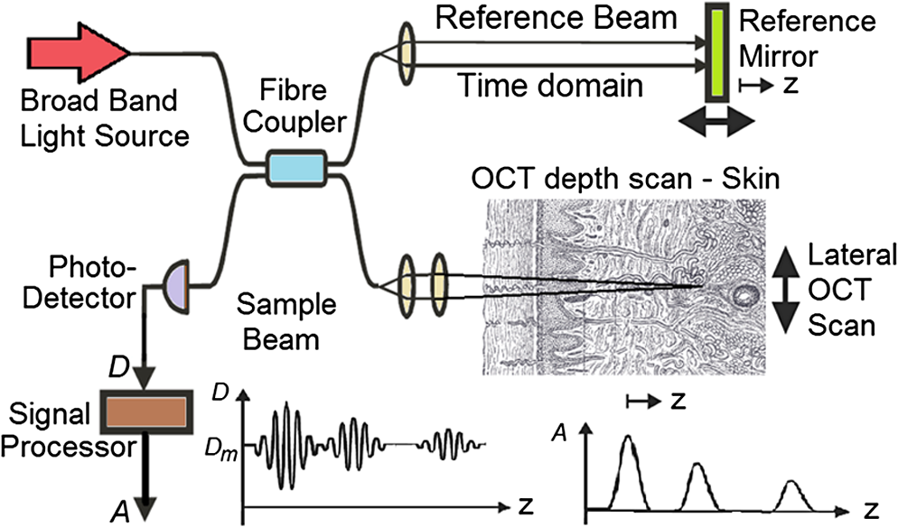
1.IntroductionOptical coherence tomography (OCT) is a two-dimensional (2-D) or three-dimensional (3-D) medical reflection imaging technique based on low coherence interferometry (LCI).1–3 As an imaging technique, the performance of an OCT system is generally quoted in terms of image resolution. That is, the lateral and axial resolution3 determine the ability of the method to discriminate between different features of a sample and provide useful information to the user. Unlike confocal microscopy, lateral and axial resolution are decoupled in OCT. Axial resolution is primarily dependent on the properties of the broadband light source that is used to illuminate the sample. Improving the axial resolution is important to detect early changes of diseases occurring at the cellular level.3 Therefore, the need to accurately quantify the axial resolution prior to OCT implementation is necessary to meet the particular resolution needed for a given histological or histopathological application. That is, the selection of an appropriate light source is critical to the validity of applying OCT imaging to a particular sample type. For Gaussian light sources, it has been proposed that the axial resolution during imaging is determined by, and equivalent to, the coherence length of the light source. The coherence length is inversely dependent on the spectral bandwidth of the light source, . As such, proposals have been expounded to improve the axial resolution of OCT imaging by producing broadband light sources with wider and wider bandwidths.3–6 However, the axial resolution limit is still quoted as the coherence length initially, which assumes a Gaussian spectrum, even if the spectrum is non-Gaussian. Realizing this, an OCT instrumentalist relies on what is believed to be a more accurate measure of axial resolution: the full width at half maximum (FWHM) of the central peak of the light source auto-correlated point spread function (PSF). In the case of these real non-Gaussian light sources, the question that needs to be answered is: what is the expected axial resolution limit and how is this limit affected by the non-Gaussian nature of the light source spectrum? These are important unresolved questions, as some proposed light sources can add considerably to the cost of implementing high resolution OCT systems, and also introduce other effects such as satellite peaks that obscure the precise nature of the imaged interferogram in an A-scan.7 The main goal of this paper is to examine the effects of light source spectral distribution on the predicted axial resolution for a common real sample model structure, in order to develop an understanding of these effects in interpreting what light source would be appropriate for different imaging applications. An LCI model has been developed that provides modular functionality so that the effect on the generated interferogram of different samples, optical delay lines (ODL), and light source characteristics could be investigated.8,9 More recently,7 the OCT model was improved to characterize and compare the effect on PSF resolution of ideal multi-Gaussian broadband light sources, which mimic the spectral characteristics of superluminescent diodes (SLDs), a typical and more affordable OCT light source. Using a further improvement of this time-domain OCT model, the present investigation extends previous research7 by demonstrating the effect of real light source spectra on the source’s PSF and interferograms of a virtual one-dimensional (1-D) epidermal model using a simulated reflective translating ODL. The purpose of this simulation research was to compare real SLD source empirical resolution and expected resolution; the latter being determined, first, from the coherence length () of the SLD spectrum, and second, from the FWHM of the central peak of the envelope of the Fourier transform of the SLD spectrum; the so-called axial PSF.3 Additionally, the purpose was to understand the dependence of the OCT A-scan relative axial resolution on a real SLD light source spectral shape, using a simplified 1-D virtual quasi-realistic epidermal sample model. In previous research,7 tandem Gaussian spectra were simulated, and it was observed that the A-scan resolution degraded with increasing spectral peaks and increasing spectral peak depths; that is, satellite peaks became larger and more numerous, degrading resolution. Though having exceptional bandwidth, many new sources for OCT present broad bandwidth spectra that are significantly non-Gaussian. Yet the same coherence length is misquoted as their resolution, even though the standard coherence length formula applies only to single peak Gaussian spectra. In this study, the work on simulated multiple Gaussian sources7 has been extended by investigating the empirical sample’s stratum depth resolution limit (SDRL) for the real SLD sources reviewed in that research.7 The OCT model has the ability to digitize real OCT source spectral data and generate the corresponding PSF and cross‐correlated interferogram (A-scan) of a virtual 1-D quasirealistic epidermal model. This sample model has strata thicknesses and refractive indices defined. It is more realistic than the previous research model,7 as it includes the air-tissue boundary’s significant reflection, as well as the actual dermal strata refractive indices from dermatological literature. As such, it allows comparison between the relative resolutions achieved between the SLD spectra considered. Also, it allows exploration of ways to enhance empirical stratum depth resolution by manipulating the A-scan data set. 2.Optical Coherence TomographyIn this section, the time-domain OCT method, OCT light source characteristics, and SLD characteristics that are selected and briefly reviewed in previous research7 and interferometrically investigated in this research, are reviewed more extensively. 2.1.Time-Domain OCT MethodIn OCT, a low coherent (broadband) light source is used to generate a reflection intensity map of a sample’s 2-D and 3-D cross-sections.3 In vivo, the absorption, scattering, anisotropy, and refractive index cross-section of the tissue layers dictates that a longer wavelength light (1310 nm) in the therapeutic window (800 to 1350 nm) will penetrate deeper than a shorter wavelength light (850 nm). As such, depending on the wavelength, penetration depths can vary from 2 to 5 mm.10 The trade-off between longer wavelength/better penetration and shorter wavelength/better axial resolution is necessary when choosing an OCT light source.3,6,7 The OCT generated interferogram depends on the light source, the sample characteristics, the ODL, and the interferometer’s type of optical circuit and component integrity. Figure 1 shows an in-fiber Michelson LCI generating a 1-D interferogram (A-Scan). Its application to OCT is seen in its ability to laterally scan the tissue to acquire a 2-D B-Scan and even 3-D C-scans. 2.2.OCT Light Source CharacteristicsIn OCT, axial resolution can vary from less than 1 μm to over 20 μm, depending on the light source spectral shape and the reflection profile of the tissue.11,12 For a Gaussian spectral light source, the axial resolution () is the coherence length, , of the source:3 for which is the source central wavelength and is the spectral bandwidth (FWHM) of the power spectrum. For a Gaussian spectrum, the axial resolution should be equivalent to the FWHM of the envelope of the PSF’s central peak. The envelope of this field autocorrelated PSF is equivalent to the Fourier transform of the light source’s power spectrum.3 Empirically, an OCT light source’s PSF can be determined from the autocorrelation of the interference signal detected at the output of an illuminated time-domain low coherence interferometer, when the sample is a simple total reflector, e.g., a mirror; an autocorrelation, maximal at the mirror surface and symmetrical in front and behind the mirror surface.Since the inverse Fourier Transform of a perfectly Gaussian spectrum in the frequency domain is itself a Gaussian in the time domain, such a light source is ideal for identifying layers in stratified samples using interferometry. The less Gaussian or multilobed or interdigitated the source spectrum, the more frequently satellite peaks or side lobes appear in the autocorrelated PSF.7 By combining SLDs7 or manipulating the SLD’s quantum energy band structure, it is possible to increase the source’s bandwidth, and thus possibly improve resolution [Eq. (1)]. If this bandwidth widening leads to non-Gaussian spectra with multiple spectral peaks, then the coherence length Eq. (1) does not apply. Such non-Gaussian spectra degrade both the PSF and A-Scan with additional smaller paired satellite peaks, symmetrical in the PSF.12 However, the PSF’s FWHM of the central peak is still considered to be the expected axial resolution when choosing an appropriate light source for an OCT imaging system.3 2.3.Superluminescent DiodesThe following SLDs have been digitized from scanned SLD spectra available from OCT literature. The OCT simulator’s Matlab function, ImageProc, generates the digitized SLD spectrum. It allows coordinate specification and generates a Microsoft Excel file of the spectrum wavelengths and their associated intensities. The OCT simulator then used this Excel data to generate the OCT PSF and tissue phantoms A-scan. Both measures of expected resolution, the SLD’s coherence length Eq. (1) and the FWHM of the SLD’s PSF, are tabulated in the results. These are compared to two measures of empirical resolution outlined and justified in Sec. 4. 2.3.1.Bulk SLDThe use of SLDs as light sources for OCT in 199113 was the second wave of use, with the first instance being their use in fiber-optic gyroscopes.11 These first SLDs were based on bulk semiconductor heterostructures with thick active layers, with their elemental III-V composition determining their emission spectra: InGaAsP emission 1.3 to 1.55 μm with 30 to 40 nm bandwidth; AlGaAs emission in the 800-nm band, with a 15- to 20-nm bandwidth.8 The left-skewed Gaussian spectrum [Fig. 2(a)] is shown for an AlGaAs Bulk SLD.11 Fig. 2(a) AlGaAs bulk heterostructure superluminescent diode (SLD) spectrum,11 and (b) AlGaAs single quantum well SLD spectrum.11  These spectra (Fig. 2) were digitally generated from the spectra provided in Shidlovski.11 Though the bulk SLD [Fig. 2(a)] spectral shape is similar to the previously simulated spectra,7 having no satellite peaks in its PSF, its Gaussian resolution limit from Eq. (1), the coherence length, is 17.3 μm, differing from its actual resolution, the PSF’s FWHM 22.3 μm, by 29%. 2.3.2.Single Quantum-Well SLDThe introduction of quantum-well (QW) SLDs achieved significant progress in resolution enhancing spectral broadening. The active region in QW SLDs is narrow enough for quantum confinement, such that the wavelengths emitted are determined by the width of the active region as well as by harmonic-like, subenergy bands existing in these QWs.7 This means that central wavelength and bandwidth broadening can be tailored by sandwiching a smaller band-gap semiconductor between a larger band-gap material. Spectral broadening occurs due to the increased density of states and sub-band transitions.7 While broadening increases with drive current, the spectrum can become multilobed [Fig. 2(b)], which may increase the empirical axial SDRL due to the appearance of satellite peaks in the PSF, interfering with reflected signals from adjacent strata interfaces. As the single quantum-well (SQW) SLD spectrum is bilobed [Fig. 2(b)], it is no longer Gaussian, so the coherence length Eq. (1) no longer applies. Instead, the FWHM of the SLD’s PSF central peak is considered to be the measure of the resolution limit.3 As the is 842 nm and is 48.4 nm, the is 6.47 μm from Eq. (1), whereas the PSF’s FWHM is 8.5 μm, differing by 31%. Clearly, the double peak in this SQW SLD spectrum [Fig. 2(b)] will increase the SDRL above the expected resolution relatively more than for the bulk SLD [Fig. 2(a)], as demonstrated in previous research.7 2.3.3.Multiple QW SLDBy fabricating multiple quantum wells (MQWs) of incrementally different widths, the emission spectrum can be broadened further. One example is the double QW separate confinement double heterostructure SLD, (InGa)As/(GaAl)As/GaAs)4 [Fig. 3(d)], with QWs of different widths. Fig. 3Spectra of the double quantum-well QW SLD,11 driven at (a) 170 mA, (b) 192 mA, and (c) 220 mA. (d) The conduction energy band structure schematic of the double QW separate confinement double heterostructure SLD.4  Considered are three spectra of this one SLD, with the active channel length of 600 μm driven at three injection currents: Fig. 3: (a) 170 mA, (b) 192 mA, and (c) 220 mA. The OCT simulator will demonstrate the detrimental effect, to the PSF and interferometric resolution limit per strata, the SDRL, of over driving and under driving the SLD. Based on the spectral and , the Gaussian resolution limits from Eq. (1) for Figs. 3(a)–3(c) are calculated to be 3.98, 3.83 and 4.68 μm, respectively. Figures 3(a)–3(c) have their expected PSF’s FWHM as 6.2, 5.2 and 5.1 μm, respectively; inflated above their coherence length by 56%, 36% and 9%, respectively. Though varying the QW width of a specific semiconductor species to broaden the SLD spectrum is considered in this spectral investigation, it is noted7 that varying the QW depth by varying the percentage composition of a heterostructured semiconductor will also broaden the SLD spectrum. However, such broadening can demonstrate poorer in vivo resolution, 6 μm,14 than the MQW SLD example considered from Ref. 4. 2.3.4.Single and Chirped Quantum Dot SLDsIn this section, a comparison is given between single-quantum dot (SQD) and chirped quantum dot (CQD) SLDs.5 CQD multilayers, in strain reducing QWs of varying composition, will broaden and red shift the emission spectrum, compared to the SQD spectrum, depending on the thickness and composition of the strain-reducing layers.5 The percentage of Indium in the InGaAs QWs was chirped from 9% to 15% in steps of 1.5%.5 The conduction band structure [Fig. 4(b) inset] and the digitized emission spectra of the SQD and CQD SLDs [Figs. 4(a) and 4(b)], generated from Fig. 1 of Li et al.5, are shown. Fig. 4Normalized room temperature photoluminescence spectra of (a) single-layer InAs QD SLD and (b) InAs multiple QDs in chirped InGaAs QW SLD, digitized from Ref. 5. Inset is conduction band schematic of the chirped QW SLD adapted from Ref. 5.  The Gaussian resolution of Figs. 4(a) and 4(b) is 16.0 and 10.1 μm, respectively. When excited and ground state emissions combine, a 6.1-μm coherence length results.7 In Figs. 4(a) and 4(b), their PSF’s FWHM are 20.3 and 12.8 μm, respectively, exceeding their ’s by 27%. 2.3.5.Quantum Dash SLDsThe quantum-dash (Q-Dash) is a finite-length wire-like structure with height and width similar to a quantum dot (QD), but with a length much longer than the QD.7 To test the resolution limit and verify the PSF of such an SLD, the SLD of Somers et al.15 would have been ideal. They demonstrated an InAs/InAlGaAs/InP Q-Dash SLD with spectral gain bandwidths of over 300 nm with near-Gaussian emission, though only above the “therapeutic window.” However, Ooi et al.16 presented a suitable spectrum, demonstrating an SLD with an InAs Q-Dash in an asymmetric InGaAlAs QW (Fig. 5, inset). This generated a quasi-Gaussian emission, with a bandwidth over 140 nm, peaking at 1.6 μm, at close to room temperature. Examined is the 77 K, state-filled, photoluminescence spectrum at excitation power (Fig. 5). The OCT simulator’s digitized spectrum is shown. The Gaussian coherence length, 6.46 μm, is exceeded by 15% by this SLD’s PSF FWHM of 7.4 μm. Fig. 577K state-filling photoluminescence spectra excitation power from the InAs-Q-Dash-in-QW SLD, digitized from Ref. 16. Inset: conduction band schematic of the four-stack InAs/InAlGaAs Qdash-in-QW active region; SCH, (undoped) separate confinement heterostructure.  Monolithic spatial bandgap engineering techniques using regrowth, selective area epitaxy, or quantum heterostructure intermixing have been used to further broaden the Q-Dash spectrum.16 By using suitable combinations of larger direct bandgap semiconductor materials, blue shifting the Q-Dash spectrum into the therapeutic window (800 to 1400 nm) may be possible, while still keeping the Gaussian and bandwidth spectral advantages of the Q-Dash SLD.7 2.3.6.Tandem Multi-SLDsTandem SLDs are often used to increase bandwidth significantly beyond that of the single, chirped QD, QW, or Q-Dash SLDs. Wang et al.6 demonstrate a combination of four SLDs with the given spectral characteristics [Fig. 6(a)], and their combined spectrum [Fig. 6(b)], digitized by the OCT simulator from Fig. 2 of Wang et al.6 This tandem SLD’s Gaussian coherence length is 5.3 μm.6 This is exceeded 27% by the SLD’s PSF’s FWHM of 6.75 μm. Fig. 6(a) Individual SLD spectra, adapted from Wang et al.,6 and (b) combined multiplexed SLD spectrum, used by the OCT simulator, digitized from Fig. 3 of Ref. 6.  Similarly, Cense et al.17 demonstrate a multiplexed SLD, the Superlum Broadlighter T840-HP, with a spectral bandwidth of 111 nm, centered at 840 nm. The OCT model’s digitized spectrum of the T-840 is shown in Fig. 7(a). This SLD, also characterized empirically by the OCT simulator, has a coherence length of 2.8 μm and a PSF FWHM of 3.46 μm, exceeding the coherence length by 24%. Fig. 7(a) Digitized Tandem T840-HP SLD spectrum,17 (b) digitized Tandem Q-940 Quad-SLD spectrum,4 and (c) the Gaussian spectral equivalent of (b).  Last, from the multiplexed SLD sources of Andreeva et al.4 the 4 mW Q-940 with a bandwidth of 307 nm and less than 50% flatness [Fig. 7(b)] has been selected for PSF and empirical SDRL analysis. This SLD’s coherence length is 1.3 μm, exceeding by 35% the PSF’s FWHM of 1.75 μm. The resolution expected by Andreeva et al.4 was quoted as 2.9 μm. The broad spectrum of the Q-9404 is made possible by the development of longer wavelength SLDs in the 1 to 1.1 μm range, multiplexed to older shorter wavelength SLDs. The development of these 1-μm SLDs was achieved using metal-organic chemical vapor deposition, which was used to fabricate the double quantum-well (DQW) (InGa)As/(GaAl)As/GaAs separate confinement double heterostructure [Fig. 3(d)]. Such an example is the 4.4-mW DQW SLD variant in Table 1 of Andreeva et al.,4 centered at 1027.3 nm with a 114.5-nm bandwidth, demonstrating a 4-μm coherence length. Table 1Summary of normal skin strata depths and refractive indices.
It may be possible to broaden such SLDs such as the Q-940 [Fig. 7(b)] further by multiplexing them to even longer wavelength SLDs,4 as demonstrated by the MQD SLD example [Fig. 4(b)] or the room temperature variant of the Q-Dash SLD (Fig. 5). However, these QD or Q-Dash SLDs would need to be significantly blue shifted, so that their spectra overlap with the 1.1-μm spectral edge of the Q-940. It is worth noting that Fig. 9 in Ref. 4 shows a significant lack of broadband SLDs between 1.05 and 1.3 μm. If this lack has been supplemented more recently, then broadening the Q-940 spectral bandwidth by further multiplexing SLDs with a longer NIR wavelength, below 1400 nm, may be possible. Figure 7(c) is the Gaussian spectral equivalent of the Q-940 SLD [Fig. 7(b)], equal in bandwidth and central wavelength. This spectrum will also be used to generate an A-scan of the epithelial sample so that its SDRLs can be compared to that of the Q-940’s PSF and A-scan characteristics, particularly with reference to the effect of satellite peaks. All of the above SLD expected resolutions will be tested with a quasi-real skin sample. Is this empirical SDRL resolution dependent only on the spectral shape—from which the and PSF are derived—or does the tissue’s strata reflection profile plays a more significant role in defining the empirical SDRLs defined in the generated A-scan? If the reflection profile is detrimental to this empirical SDRL, then is it possible to digitally enhance the empirical resolution to bring it closer to the expected SLD resolution; the SLD’s PSF FWHM? These questions are answered in this research along with any justification for the validity of the digital resolution enhancement techniques used. 3.TheoryThe OCT simulation models a single axial scan Michelson interferometer (Fig. 1) using a virtual translating mirror in the time domain on a virtual linear scanner as the ODL. The model was developed from low coherence interferometric first principles. It uses purely the optical and spectral physics involved in an ideal Michelson interferometer and includes the interaction with the sample. It does not involve a direct integral convolution of the PSF envelope with a series of virtual sample strata-interface delta functions scaled by strata reflectivity. The later, using only the PSF envelope, could not include the effect of full phase interference that is demonstrated by this more developed OCT model. In this study, we are interested in determining the limits of resolvability, which are affected by destructive interference in the phase modulation between reflected strata interface full phase PSFs. The virtual sample used is a 1-D stratified five layer structure with definable layer refractive indices typical of normal epithelia, from which layer reflectivities are calculated using Fresnel’s law. The sample model is a tool that is used to determine the effect of different low coherent light sources on the empirically obtained minimum depth resolution per sample stratum. In this case, because of the sample model’s simplicity, this will be a relative depth resolution. As long as all the real SLD light source spectra are applied to the same refractive index layer epidermal model, comparison of the resolution limit between the A-scans of the light sources is possible. Previous research used this model with simulated single and tandem Gaussian spectra. It demonstrated that the presence of satellite peaks in the PSF-degraded resolution are due to multiple peaks in the spectra.7 To corroborate these results using real OCT light source spectra, this research used the same LCI model, modified to allow the scanning and digitizing of any real low coherent light source’s spectrum. The model presented here includes the effect on the resulting A-scan by the refractive index profile of the sample strata, resulting in the slowing of the speed of the light in each layer proportional to the refractive index. However, for this research, for direct comparison between the actual layer depths and those in the A-scans, the model’s ability to account for the effect of layer refractive index on light speed in the tissue has been suspended. The following sections detail the equations of the optical model developed. This model, which has been formulated previously,8,9 has been reformulated into a more effective model from the point of view of sample application and real light source spectral application from that of the recent previous model.7 3.1.Modeling the Light SourceSuppose that a light source emits a continuous distribution of wavelengths whose amplitude, , is a function of the wavelength (the wavelength in the surrounding medium, typically air); that is For example, if the distribution of wavelengths has a Gaussian form we have where is the peak amplitude, is the central/peak wavelength, and is the spectral bandwidth (FWHM intensity). The laser power is given by .3.2.Modeling Light in the InterferometerThe distribution of wavelengths is first passed through a 50% mirror, with half of the light reflected and half transmitted. The result is a reflected (R) and transmitted (T) wave with amplitude distributions, The transmitted wave, considered to be the sample arm of the interferometer, travels to a multilayered surface consisting of partially reflecting interfaces, the phantom structure to be imaged. The transmitted wave goes through transmission and reflection at each interface. Upon returning from the multilayered interface, the transmitted wave is reflected by the 50% mirror to the detector. The reflected wave, considered to be the reference arm of the interferometer, travels from the 50% mirror to another reflector which is moved incrementally (i.e., no Doppler effect) before being reflected back through the 50% mirror (transmitted) to a detector. Once the original light source is split, it becomes important to keep track of the virtual distance traveled by each wave, as any difference will be associated with a phase shift and therefore a change in the interference pattern. The virtual distance, as opposed to the actual distance, takes into consideration changes in the velocity of the wave as it passes through layers with different refractive indices, which is relevant to the generation of real LCI A-scans. The total distance traveled by the transmitted wave which reflects off the top surface/interface of the multilayered structure is denoted as . The thickness of the ’th layer in the sample [i.e., the distance between the th and th interface] is denoted , for . Hence, the total distance traveled by the wave reflected off the ’th surface of the sample is given by whereas the virtual distance traveled by these waves is given by where is the refractive index of the medium in front of the sample and is the refractive index of the ’th layer of the sample. The total distance traveled by the reflected wave is denoted by . Note that and , since the waves traveling these distances are only transmitted through the surrounding medium.The reflectivity of the ’th interface of the sample is denoted by and is given by Fresnel’s law as The reflectivity of the reference arm mirror is denoted by (although typically ). We have assumed that the contribution of waves which are reflected off multiple interfaces within the multilayered structure is negligible. Therefore, it makes sense to decompose the detected component of the sample transmitted wave into parts corresponding to each of the reflecting surfaces. Hence, we have The final amplitude distribution of the reflected wave is In the interest of notational convenience, we define a reflectivity factor Then the amplitudes of the transmitted and reflected waves can be expressed as 3.3.Modeling the Detected Cross CorrelationHaving defined expressions for the amplitudes of the interfering waves, we now consider the interference of these waves. Without loss of generality, we can represent all waves using a sine function with the origin at the detector. The expression for the ODL reflected wave is while for the (originally) transmitted sample components we have where is a phase shift indicator function given byNote also that . For the sake of simplifying notation, let Then we can write equations for the ODL () and sample (), The resultant wave arriving at the detector is therefore given by whereIt follows that the amplitude of the resultant wave is given by and hence that the total intensity of detected light over all wavelengths is given byBy simplifying the integrand in Eq. (20), the intensity expression can be expressed in a more convenient form, so that the intensity at the detector can be expressed as whereNote that if is a Gaussian spectrum as per Eq. (3), then The expression given in Eq. (21) separates the intensity into a constant offset component (i.e., constant for a specific sample structure with fixed distances and reflectivities ), and an interference component for each of the layers given by . The coefficient contains only information relating to layer reflectivities, whereas the function contains the information related to the layer virtual distances. 4.MethodThe method used to set up the simulation parameters is described below. Also considered is the technique used for improving the empirical A‐scan’s SDRL, as well as a brief justification for the technique. 4.1.Virtual Skin Model ParametersRigorous models of skin can be quite complex as skin is irregularly shaped, has hair follicles, glands, and blood vessels, is inhomogeneous, cellularly multilayered, and has scattering, absorption, and anisotropic properties.26 As OCT has demonstrated benefit to the detection and monitoring of various skin pathologies, therefore, the application of OCT in a dermatological context is of interest in this research. A sample structure has been developed from an ideal phantom structure7 [Fig. 8(a)] to a quasirealistic skin model [Fig. 8(b)]. This has been implemented for context only, and not for realistic application. The old and new models are compared in Figs. 8(a) and 8(b), respectively. The layer depths given are typical for a normal epithelium. These layers may be expanded due to pathological hyperplasia, especially for the Stratum germinatum. Fig. 8(a) Previous sample structure7 and (b) quasi-realistic epidermal structure identifying layer depths and refractive indices typical of normal skin tissue. 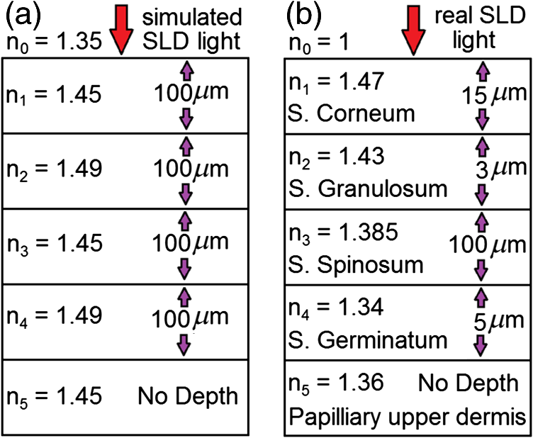 The sample layer thicknesses given in Fig. 8(b) are typical for normal epithelia synthesized from Table 1. So that the SDRLs of the selected SLDs can be tested, the tissue model layer thicknesses differed from Fig. 8(b) and differed between SLDs because the PSF of each SLD spectrum differed between SLDs, resulting in different SDRLs for each SLD, i.e., a different sample layer thicknesses for each SLD. The acquisition of SDRLs requires the incremental change in each stratum thickness and repeated simulation, until the SDRL is reached for each stratum for a particular SLD source. However, the tissue models’ layer refractive indices remained unchanged [Fig. 8(b)]. Table 1 identifies normal skin layer parameters and Table 2 synthesizes the generic parameters used in the epidermal skin model as identified in Fig. 8(b). Table 2The normal skin parameters used for each SLD A-scan.
Of interest is the identification of the early stage of skin cancer, of which melanoma is one example. The cancer is produced by melanocyte hyperplasia in the stratum germinatum and so identifying the thickness of this layer is of interest. As such, the OCT light source needs to be able to resolve the stratum germinatum in contrast to adjacent layers. Figure 9(a) shows typical normal skin histology in contrast to the melanomatous in Fig. 9(b). Figure 9(b) shows a dysplastic melanoma nodule, 35 μm deep and 50 μm laterally. Note its cellular scarcity compared to the concentration of cells in the surrounding stratum germinatum. With less structural “scaffold” and more fluid, the refractive index of the nodule may be closer to that of water (). Fig. 9(a) Heamatoxylin and Eosin (H & E) stained skin histogram, identifying cellular layers in normal skin (adapted from Ref. 27) and (b) H & E micrograph: melanoma dysplastic nodules with distended melanocytes, showing melanin content (adapted from Ref. 22).  To relate the layer thicknesses and refractive indices of typical skin tissue to those used to test the SLDs, Table 1 surveys typical values from the literature. Due to the interest in using OCT for skin pathology characterization, the table outlines the tissue parameters of the skin layers indicated in Figs. 9(a) and 9(b) that are typical for normal skin [Fig 9(a)]. Most epithelial pathologies express as hyperplasia. This increases the epithelial strata thickness. Therefore, the normal strata thickness is the lower limit of resolution. The parameters of the skin model used by this OCT model, having been synthesized from Table 1, are presented in Table 2. Only four epithelial layers are considered, having a total depth depending on the sum of the depths (a) to (d) in Table 3 in the Results section. Stratum Lucidium is omitted as it only occurs in the sole and palm. Table 3SDRL for SLDs by skin strata: in descending depth order: stratum corneum (SC), stratum granulosum (SGr), stratum spinosum (SS), and stratum germinatum (SGe), for each (A) SLD A-scan and (B) FSI-subtracted A-scan.
4.2.SLD PSF and InterferogramsThe envelope of the SLD’s PSF is the Fourier transform of the light source’s power spectrum.3 The full PSF with phase information, not just the envelope, was determined for each source as the autocorrelation of the interference signal detected at the output of the interferometer using a single reflective surface (a mirror) as the sample. This autocorrelation is maximal at the mirror surface and symmetrical in front of and behind the mirror surface. Here, the sample needed to be defined as a virtual mirror; as such the virtual sample surface was defined as 99.9996% reflective. The sample was then scanned by the virtual translating mirror ODL above and below the air-mirror interface to generate the symmetrical full PSF interferogram. Using the appropriate quasirealistic 1-D in vivo skin sample geometry from Table 2, each SLD source example from Sec. 2.3 was used to generate an A-Scan of the sample. Then the two empirical measures of axial resolution are described in Sec. 4.3 (defined as methods A and B). For clarity of determining the maximum points from the full in-tissue sample A-scan after method A and B treatments, the central intensity axis about which the A-scan modulated symmetrically was located and the intensities below this axis were flipped symmetrically above this axis. To clarify, as the A-scan was approximately symmetrical, the average intensity of the A-scan was the axis of symmetry. By subtracting this average intensity from each A-scan intensity, the absolute value was taken and the positive peak A-scan was arrived at. This mathematical treatment flipped the minimum peaks vertically, so that the maximum extension of each A-scan peak became more obvious. Table 3 summarizes four estimates of resolution for each SLD: each SLD’s coherence length, Eq. (1), each SLD PSF’s central peak FWHM expected resolution, and its minimum layer thickness resolution limit for each layer depth (SDRL) using methods A and B described in Sec. 4.3. 4.3.Methods for Determining the Empirical Axial SDRLIn order to evaluate each light source, it was necessary to define how the axial resolution limit was obtained. For the purposes of this investigation, the axial SDRL was defined as the minimum layer thickness per stratum for which the simulated stratum interface position in the A-scan was within of the actual layer surface position, predefined in the epidermal sample model. This required the strata thicknesses to be independently varied until a minimum depth was reached per stratum that met this tolerance. This then gave the minimum resolvable stratum thickness; i.e., the empirical SDRL. There was particular interest in investigating a new technique that manipulated the A-scan to remove significant reflection from the virtual skin phantom surface. To this end, two methods to acquire the empirical axial SDRL were defined and their SDRLs compared: Method A: Using the A-scan alone to determine the SDRL. Here, the resolution limit was identified in each A-scan for each source by incremental expanding each layer thickness independently until the minimum layer thickness resolution limit was reached; i.e., when the empirically resolved layer thickness equated with the expected layer thickness ; the expected resolution being the FWHM of the PSF’s envelope central peak. Method B: Mirroring the A-scan’s front surface interferogram (FSI), i.e., the front surface full phase PSF—the portion of the A-scan extending above the surface—back onto the subsurface A-scan and then subtracting this FSI from the portion of the A-scan below the sample surface. This method was exactly the same as method (A) with the exception that only the A-scan’s FSI was digitally subtracted from the A-scan itself. This then exposed the buried PSFs of the lower strata interfaces which had been masked by the FSI. This procedure removed the large reflection peak that existed at the surface of the generated A-scan which was caused by significant surface reflection at the air–tissue interface. It is important to note that, though method (B) will be demonstrated by manipulating the simulation results of the surface-symmetrical A-scans, it needs to be verified using a real surface symmetrical A-scan or an A-scan that demonstrates the full FSI above the sample surface for real OCT postprocessing applications. Clearly with an undulating skin surface, the extent of the subtracted portion of the surface PSF above the surface will differ between adjacent A-scans. However, as long as the full half of the FSI above the surface is present in each A-scan and the A-scan depth in the tissue is equal to or greater than the extent of the FSI above the surface, FSI subtraction would eliminate the surface “glare.” A justification for the subtraction of the FSI from the A-scan, rather than a deconvolution of the FSI from the A-scan, is given in the following section. 4.4.Justification for the FSI-Subtracted A-scan TechniqueThe FSI is subtracted from the subsurface A-scan in order to allow determination of the empirical depth resolution limit by removing the intense surface reflection that masks the less reflective subsurface strata. The justification for this manipulation is based on the fact that the variable component of the detector intensity is just a linear sum of interference terms associated with each interface of the sample structure, as represented by Eq. (21). That is, each term in the sum is independent of the position of other layers in the sample, so the subtraction of the term corresponding to the top stratum surface layer does not impact the location of peaks in the intensity function resulting from the other strata. In a previous study,7 the sample model consisted of a five layer structure with equal layers thicknesses of 100 μm and defined constant refractive indices, as shown in Fig. 8(a). As such, the effect of any front surface (air-sample interface) reflection was negligible, as the PSF of all the light sources considered both in this current study and the previous study have PSFs that extend less than 40 μm spatially on each side of the PSF central maximum. For Gaussian light sources, this PSF spatial extension is considerably less. Hence, although the air-sample interface reflection appears in the A-scan, its effect on subsequent interface peaks for subsurface strata will be insignificant. In this study this condition is not satisfied, as the first few subsurface interfaces often lie within the spatial range of the source PSF from the air-sample interface. Hence, there is a need to remove the surface reflection peak in order to examine the effect of light source resolution on the ability to image the lower strata. Note that in a real physical measurement, the surface reflection peak would be present and would need to be removed or the observed A-scan modified to allow the determination of the underlying sample structure. It is worth noting that although the terms of the intensity Eq. (21) are independent with respect to the layer positions, the reflectivities of the preceding layers do influence the magnitude of the intensity components from each layer. This, however, would only influence the vertical extent of the A-scan, and not the horizontal extent (i.e., position information). It is also worth noting that the intensity Eq. (21) can be thought of as the convolution of the sample structure with function . Furthermore, the function is the Fourier transform of the function where is the wave number, and is the source amplitude as a function of wavelength.4.5.Current OCT ModelThis version of the OCT model allows the choice of a sample with as many layers as required—five layers in this research—and only two sample layer characteristics—layer thickness and refractive index. Though it is capable of presenting refractive index corrected stratum positions in the A-scan, this ability was suspended for this research, so that actual SDRL information could be directly read from the A-scan. Having the added flexibility of defining a Gaussian source or scanning in a real source spectrum as well as defining an ODL, this version of the OCT model can be used to study the effects of OCT light sources,7 ODLs,9 and sample types on OCT operation. At this early stage of the model’s development, effects of dispersion, internal reflection, heating, polarization, tissue absorption, and scattering anisotropy have not been incorporated in the model. These occur because a real OCT optical circuit presents imperfections at every point in the interferometric circuit. Instead, the sample’s structure is simply defined by two parameters: strata refractive indices and thicknesses. But as explained earlier, as long as the sample layer refractive indices remain constant, the effect of the light source shape on A-scan relative resolution can be compared between sources. This allows ranking of the sources in order of increasing SDRL, with the best, most resolved sources at the top of the ranking. Furthermore, this research is mainly focused on the comparison of different SLD effects on their relative resolution using a quasirealistic epidermal model, so our predicted axial resolutions are the upper limits of resolution. 5.Results and DiscussionThe results are presented so that comparisons can be made between the two methods used to acquire the SDRLs, the standard measures of OCT light source resolvability and the normal stratum depths. This is carried out in order to establish any advantages in using the second method: subtracting the FSI from the A-scan. First, the results are summarized in two tables: In Table 3, the resolution limit by stratum type for each SLD for A-scan-only and FSI-subtracted A-scan processing methods; and in Table 4, the average resolution limit and 95% confidence interval across all strata for each SLD type and each processing method. Table 4Summary of average SDRL and SDRLs relative to their expected axial resolution from Table 3.
Second, Table 3 results are graphically summarized by resolution limit dependence on SLD type for each stratum type with comparison to normal stratum thickness, using A-scan-only and FSI-subtracted A-scan data processing methods. Then, each SLD is discussed separately with reference to their Table 3 results and graphical summary entries in Fig. 10. Fig. 10Depth resolution dependence on SLD type and digital processing method. (a) stratum corneum (at surface), (b) stratum granulosum, (c) stratum spinosum, (d) stratum germinatum; normal stratum depth range is indicated.  Third, each SLD is discussed separately with reference to their Table 3 results, their Fig. 10 graphical summary, and three interferograms: (a) the SLD’s PSF, (b) the SLD’s A-scan showing SDRLs, and (c) the SLD’s FSI-subtracted A-scan showing SDRLs. The stratum depth resolution for strata thinner than their resolution limit are either not demonstrated as peaks in the A-scan (not resolvable) or the peak of the stratum position indicated in the A-scan is significantly different () to the stratum depth defined in the sample. These interferograms are accompanied by a graph that summarizes the SLD’s SDRL dependence on stratum type, with comparison to the typical estimates of resolution: the SLD’s coherence length and the SLD’s PSF central peak FWHM. Finally, the average SDRL dependence on SLD type across the four epithelial strata, including their 95% confidence intervals, are summarized both in Table 4 and graphically in Figs. 23 and 24. This is for each SLD’s A-scan average SDRL with and without FSI subtraction. All references in this results section to the average SDRLs and the average SDRL relative to the expected SLD axial resolution, the PSF’s FWHM, come from Table 4, tabulated in Sec. 5.9. 5.1.SDRL Summary by StratumTable 3 summarizes the SDRL for each stratum by SLD type. The coherence length and SLD PSF FWHM expected resolution values have also been calculated. Figure 10 makes the comparison between the resolution limits of each SLD, using the A-scan and FSI-subtracted A-scan, and the normal depth range for each epithelial stratum. Figure 10 shows how applicable each SLD is for skin OCT in terms of axial resolvability. To be acceptable as a light source with resolution appropriate for epidermal imaging, the SLD’s SDRLs must fall inside or below the normal range for ALL strata [Figs. 10(a)–10(d)]. Within the limitations of this simulation and the sample definition, with just the A-scan, only the Quad SLD Q940 is suitable for OCT imaging of skin. With FSI subtraction from the A-scan, two more SLDs qualify: the optimally driven (192 mA) MQW SLD (5.3b in Fig. 10), and the Cense17 tandem SLD (5.7b in Fig. 10). This clearly demonstrates the benefit of the FSI-subtracted A-scan technique for collapsing the SDRLs closer to the expected axial resolution of each SLD. Clearly, the FSI-subtracted A-scan technique has advantages over just using the A-scan. It eliminates the significant surface reflection, allowing subsurface PSFs to be expressed and so allowing the SDRLs to come much closer to the expected resolution for each SLD, especially for the uppermost stratum’s SDRL. 5.2.Bulk SLDThough the Bulk SLD PSF [Fig. 11(a)] has no satellite peaks similar to Gaussian spectra previously simulated,7 since the spectrum was left skewed [Fig. 2(a)], agreement with the expected measures of resolution differed significantly. The average empirical SDRL (bulk SLD in Table 4) for the A-scan-only and FSI-subtracted A-scan methods were significantly inflated above the coherence length (), but not significantly different from the SLD’s PSF FWHM (22.3 μm). However, for the A-scan [Fig. 11(b)] and the FSI-subtracted A-scan [Fig. 11(c)], the SDRL for all four strata and the bottom three strata, respectively, exceeded the SLD’s PSF FWHM. However, though the FSI subtracted A-scan’s average SDRL was less than not subtracting the FSI , it was statistically not significantly different. Fig. 11AlGaAs bulk SLD11 with . (a) SLD full phase PSF, full width at half maximum , (b) A-scan, and (c) FSI subtracted A-scan, of minimum SDRL sample.  Clearly the benefit of FSI subtraction is demonstrated only for the surface stratum, as the bulk SLD spectrum is significantly Gaussian, expressing no satellite peaks in the PSF, which would otherwise also degrade the A-scan SDRL for the lower strata. The lowest stratum increases its SDRL for both the A-scan and the FSI-subtracted A-scan methods, because this stratum is least reflective and is suppressed by the larger adjacent peak. Epidermal definition using this SLD with OCT in normal tissue of the significantly thinner stratum granulosa [Fig. 10(b)] and stratum germinatum [Fig. 10(d)] will not be possible, because there can be no depth contrast between normal histology and pathology. Even early-stage moderate hyperplastic melanomacytic nodules in the stratum germinatum (Fig. 9) may not exceed the SDRL of this SLD for this stratum. 5.3.Single-Quantum Well SLDThis SLD generated satellite peaks in the PSF [Fig. 12(a)] due to the double peak in the SLD spectrum [Fig. 2(b)], as predicted by the double Gaussian peak spectra simulated in previous research.7 The obvious difference in SDRL between the method using the A-scan only [Fig. 12(b)] and the method using the FSI-subtracted A-scan [Fig. 12(c)] is due to three significantly large pairs of satellite peaks that extend over 30 μm from the PSF center [Fig. 12(a)]. This is particularly obvious for the subsurface part of the FSI [Fig. 12(b)] expressing two of the three satellite peaks significantly larger than the underlying strata peaks. Furthermore, the three satellite pairs associated with each interface PSF present a zone to either side of each interface that restricts the SDRLs’ ability to be any closer to the expected SQW SLD resolution (Table 3), that is, its PSF’s central peak FWHM being 8.5 μm. However, all SDRLs are significantly reduced as soon as the intense FSI is subtracted from the subsurface A-scan. This collapses the inflation of the average SDRL above the expected SLD resolution, from () down to only (). Fig. 12SQW AlGaAs SLD11 with . (a) SLD full-phase PSF, FWHM=8.5 μm, (b) A-scan, and (c) FSI-subtracted A-scan, of minimum SDRL sample. 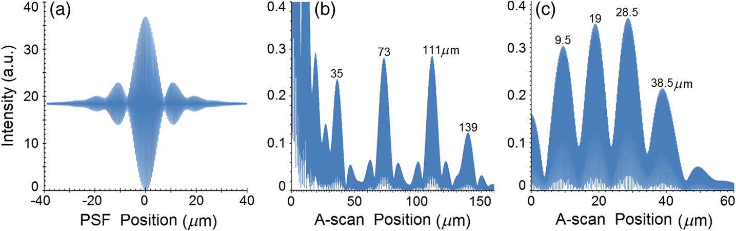 The average SDRL, for the A-scan-only, , and FSI-subtracted A-scan, , were significantly inflated above this SLD’s coherence length (6.5 μm), and its PSF FWHM (8.5 μm). However, similar to the previous SLD, the SDRL for the FSI-subtracted A-scan was significantly less than when the FSI was not subtracted. Due to the increased density of states in this SLD’s SQW and its sub-band transitions,7,11 the actual empirical SDRLs improved significantly above that of the bulk SLD [Fig. 11(b)] only when the FSI was subtracted; their average SDRLs were not statistically significantly different without subtracting the FSI from the A-scan. However, early melanoma-hyperplasia false positives may be indicated in OCT B-scans using this SQW SLD, since normal stratum granulosa and stratum germinatum, the second and lowest epithelial strata, thicknesses are 3 to 7 μm [Figs. 10(b) and 10(d)], which is 1 to 2 squamous cells thick. 5.4.Multiple QW SLD with Variable Drive CurrentFurther spectral broadening was achieved using chirped width double QW SLDs [Fig. 3(d)]. Results are presented as a function of the SLD drive current: Fig. 13 shows the under-driven case (for a drive current of 170 mA, 5.4A in Table 3), Fig. 14 shows the optimally driven case (192 mA, 5.4B in Table 3), and Fig. 15 shows the over-driven case (220 mA, 5.4C in Table 3). Fig. 13The 170 mA driven MQW SLD4 [band structure Fig. 3(d)] with . (a) SLD full-phase PSF, , (b) A-scan, and (c) FSI-subtracted A-scan, of minimum SDRL sample.  Fig. 14The optimally driven, 192 mA, MQW SLD4 [band structure Fig. 3(d)] with . (a) SLD full-phase PSF, , (b) A-scan, and (c) FSI-subtracted A-scan, of minimum SDRL sample.  Fig. 15The 220 mA driven MQW SLD4 [band structure Fig. 3(d)] with . (a) SLD full-phase PSF, , (b) A-scan, and (c) FSI-subtracted A-scan, of minimum SDRL sample.  Under-driving this SLD at 170 mA gave a resolution inflation of () above 6.2 μm, for an average SDRL of () (Table 4), only after subtracting the FSI from the A-scan [Fig. 13(c)]. Without subtracting the FSI, the average SDRL inflation for this under-driven SLD was () above 6.2 μm, for the average SDRL of (Table 4). This SLD, driven at the intermediate current of 192 mA (Fig. 14), gave the least average SDRL inflation, () above 5.2 μm, having the best average SDRL, (), only after subtracting the FSI from the A-scan [Fig. 14(c)]. Without subtracting the FSI, the average SDRL inflation for this SLD, optimally driven at 192 mA, was () above 5.2 μm, for an average SDRL of . Over-driving this SLD at 220 mA resulted in the two largest pairs of satellite peaks [Fig. 15(a)], which especially affected the weakest reflecting lowest stratum, pushing all the SDRLs deeper. This resulted in a resolution inflation of () above 5.1 μm, for an average SDRL of , only after subtracting the FSI from the A-scan [Fig. 15(c)]. Without subtracting the FSI, the average SDRL inflation for this over-driven SLD was () above 5.1 μm, for the average SDRL of . Note that the resolution limits of the under-driven SLD (Fig. 13) and over-driven SLD (Fig. 15) are not statistically significantly different. Furthermore, the average SDRL for all three drive current conditions for the A-scan only are not significantly different due to the large variation of the SDRLs between strata [Figs. 13(b), 14(b), 15(b)]. However, when the FSI is subtracted from the A-scan [Figs. 13(c), 14(c), 15(c)], the average SDRLs of the under-driven and over-driven MQW SLD are not significantly different, while they are clearly larger than the average SDRL of the optimally driven MQW SLD. In summary, for QW SLDs, the resolution limit “sweet spot” is drive current dependent, while this is not the case for bulk SLDs.11 Furthermore, to gain the SDRL benefit for this MQW SLD, the FSI needs to be subtracted from the subsurface A-scan. Note how stable, and close to the expected SLD axial resolution of 5.2 μm (Table 3) the optimally driven SLD is after the FSI was subtracted from the A-scan. Subtracting the FSI from the A-scan has the added benefit of advancing this SLD to being applicable for OCT epithelial imaging. Having an SDRL of is not significantly greater than the normal stratum germinatum thickness of 3 to 6 μm [Fig. 10(d)]. Depending on the melanoma nodule’s degree of aqueousity, normal stratum germinatum may be contrasted from premalignant nodules, clearly visible in the hematoxylin and eosin histogram (Fig. 9). However, it would be better if the SDRL of the SLD fell below the lower limit of the normal thickness range for this thinnest stratum [Fig. 10(d)], because if the stratum was actually thinner than the SDRL, which is , the stratum would not be resolved. 5.5.Single Layer Quantum Dot SLDDue to the smaller peak in this SQD SLD’s spectrum [Fig. 4(a)], symmetrical humps appeared in the SLD’s PSF [Fig. 16(a)]. These resulted in four symmetrical ridges on either side of each stratum peak in both interferograms [Figs. 16(b) and 16(c)]. Fig. 16Single-layer InAs QD SLD5 at room temperature with . (a) SLD full-phase PSF , (b) A-scan, and (c) FSI-subtracted A-scan, of minimum SDRL sample.  The obvious difference in SDRL between the A-scan [Fig. 16(b)] and the FSI-subtracted A-scan [Fig. 16(c)] was due to the significantly large FSI that inhibits the expression of strata peaks lower in the sample. Due to this causing a large variation in the SDRL, the average SDRL for the A-scan [Fig 16(b)], of , was not significantly different from the expected resolution (Table 3), being 20.3 μm. When the FSI was subtracted from the A-scan, the average SDRL collapsed to . Though not significantly different from the A-scan average, clearly the FSI subtraction benefited the average SDRL, reducing it 16%. Furthermore, after FSI subtraction, the SDRL was reliably constant across all strata. As was the case for the bulk SLD and the single QW SLD, the SDRLs were too large, greater than 21 μm, for useful application to premalignant skin pathology diagnosis. False positives in OCT B-scans are possible, because of the thinness of the granular (3 to 6 μm) and germinal (4 to 7 μm) epithelial strata20 (Table 1). 5.6.Multiple QDs in Chirped QW SLDFigure 17(a) shows the full-phase PSF for this multiple QD SLD, for its given spectrum [Fig. 4(b)]. The small satellite pair, occurring 20 μm to either side of the central PSF peak, is seen in the A-scan [Fig. 17(b)] to the left of the first 36-μm stratum peak. Figure 17(c) shows the benefit of FSI subtraction, particularly for the uppermost stratum. Fig. 17InAs multiple QDs in chirped InGaAs QW SLD5 at room temperature [Fig. 4(b)] with . (a) SLD full-phase PSF, , (b) A-scan, and (c) FSI-subtracted A-scan, of minimum SDRL sample. 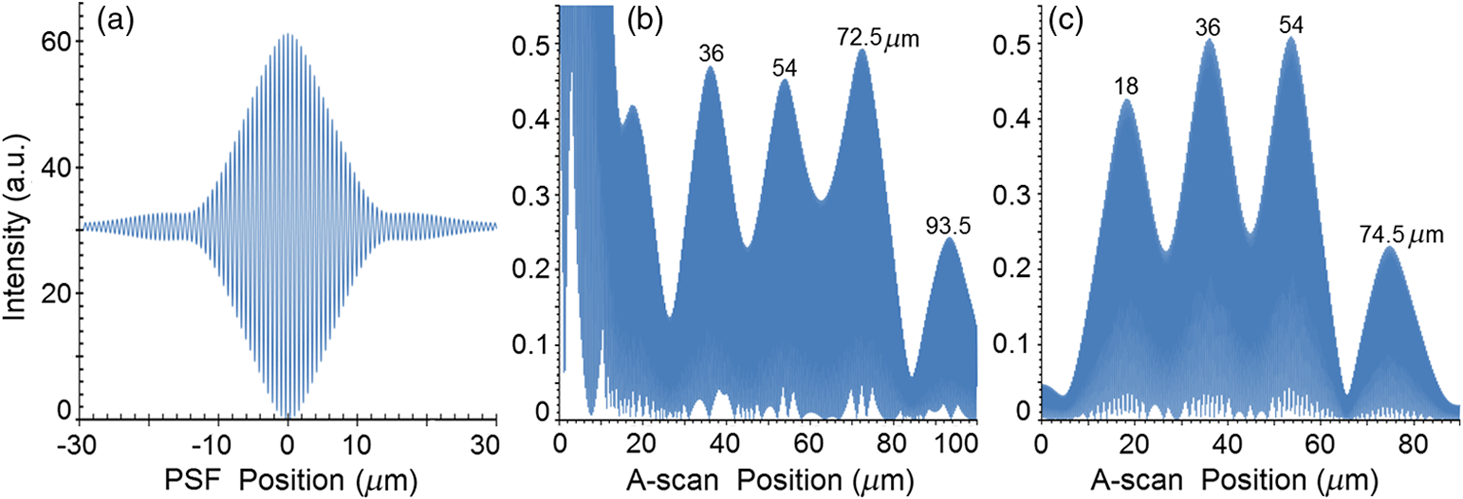 In contrast to the SQD SLD, both the multiple QD and the chirped QWs seen in this SLD’s electronic band structure [Fig. 4(b) inset] broadened and red shifted this SLD’s spectrum,5 resulting in a right-skewed Gaussian shape [Fig. 4(b)]. With this broadening, the small peak apparent in the SQD SLD spectrum [Fig. 4(a)] was eliminated, reducing the average SDRL, relative to the SQW SLD, by 11% and 5%, with and without FSI subtraction, respectively. Noted was the lack of false layer peaks in the FSI-subtracted A-scan [Fig. 17(c)]. However, in the same way that the bulk SLD had a skewed spectrum [Fig. 2(a)], this right skewed SLD spectrum [Fig. 4(b)] generated an average SDRL, with and without A-scan FSI subtraction, of and , respectively (Table 4). This was an inflation above the expected resolution (Table 3) of and , respectively (Table 4). Clearly, only the top stratum’s SDRL has been improved by the FSI subtraction since the FSI is adjacent to this stratum, and satellite peaks are not significant in the PSF [Fig. 17(a)]. The SDRLs are still not small enough to be useful in distinguishing normal from pathological epithelia. As a result, this SLD may indicate false-positive B-scan premalignant dysplastic epithelia because of the normal epithelial strata thinness, as mentioned for the previous SQD SLD and indicated in Figs. 10(b) and 10(d). 5.7.Q-Dash in Asymmetric QW SLDUnlike the previous Q-dot SLDs, this SLD does have a significantly large pair of satellite peaks due to its two-peak spectrum (Fig. 5), caused by a combination of the asymmetric QW and Q-dash band gaps (Fig 5 inset). This results in the expression of the SLD’s FSI with a satellite peak [Fig. 18(b)] larger than the strata peaks below it. Though this SLD spectra was quasi-Gaussian, the presence of the double peak resulted in its average SDRL in the A-scan, with and without FSI subtraction, being inflated above the expected resolution (7.4 μm, Table 3) by and , respectively, being and , respectively (Table 4). As usual, the Gaussian coherence length from Eq. (1) is never a good estimate of resolution. In this case, it is only 6.5 μm (Table 3). Fig. 18InAs Q-dash-in-QW SLD16 at 77 K and excitation power, with . (a) SLD full-phase PSF, , (b) A-scan, and (c) FSI-subtracted A-scan, of minimum SDRL sample.  The FSI-subtracted A-scan was free of false-strata satellite peaks, resulting in clear, well separated strata peaks [Fig. 18(c)]. Clearly, FSI subtraction improves each SDRL further into the sample compared to the Q-dot SLDs above, for which only the front stratum benefited. For this SLD, even the bottom strata’s SDRL was slightly improved. Is this SLD appropriate for OCT dermal application? Unfortunately, even with FSI subtraction, this SLD may also generate B-scan malignant dysplastic epithelial false positives due to the individual SDRLs exceeding the normal thickness of the stratum granulosum and stratum germinatum [Figs. 10(b) and 10(d)], as was the case in the above SLDs. Water absorption will also reduce sensitivity and resolution in an OCT A-scan. This SLD’s spectral width crosses the near infrared wavelength region at which water absorption is significant. In a real in vivo scan, this would result in reduced light source penetration depth and reduced ballistic reflection intensity from each interface. This would result in more interference effects from the FSI on lower interface reflections, so removing the FSI would still be advantageous. 5.8.Multiplexed SLDsIn this section, we compare three types of tandem SLDs. Their A-scan, PSF and SDRL’s dependence on stratum type are presented. First, Wang et al.6 demonstrated the advantage of combining four Gaussian SLDs, which was immediately seen in the improved resolution limit being greater than each constituent SLD [Fig. 6(a)]. However, this combined spectrum [Fig. 6(b)] now had a peak triplet, which, as predicted previously,7 resulted in two major pairs of satellite peaks appearing in the PSF [Fig. 19(a)]. Because of this, significant satellite peaks were evident in the A-scan [Fig. 19(b)], some larger than the strata peaks. The effect of these satellite peaks disappeared when the FSI was subtracted from the A-scan [Fig. 19(c)]. These satellite peaks restrict any thinner sample layer definition in both the A-scan and the FSI-subtracted A-scan. However, though the bandwidth was 145 nm, the average SDRL with and without FSI subtraction was and , respectively. These represent an inflation of and , respectively (Table 4), above 6.75 μm, the expected resolution (Table 3). Fig. 19Quad-SLD6 with . (a) SLD full-phase PSF, , (b) A-scan, and (c) FSI-subtracted A-scan, of minimum SDRL sample. 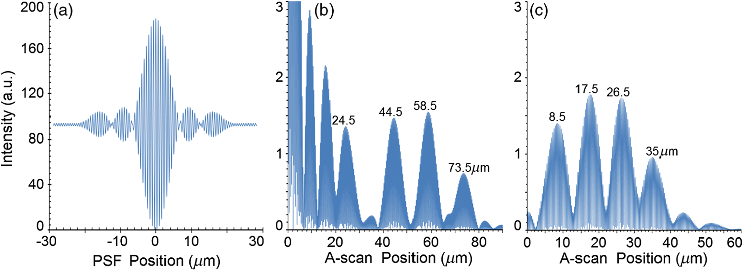 Comparison of the individual SDRLs and their expected resolutions (Table 3) show that the FSI-subtracted A-scan results are superior by being closer to the expected resolution and much more stable across strata. The gradual decrease of the SDRLs downward through the sample shows the reducing detrimental effect of the FSI interference deeper into the sample. Is this SLD appropriate for OCT dermal application? Unfortunately, even with FSI subtraction, this SLD may also generate B-scan malignant dysplastic epithelial false positives, due to the individual SDRLs exceeding the normal thickness of the stratum granulosum and stratum germinatum, as was the case in the above SLDs. Second, the next multiplexed SLD was presented by Cense et al.17 They reported on the Superlum Broadlighter T840-HP SLD, illuminating in the 800- to 900-nm spectral band [Fig. 7(a)]. This SLD spectrum was particularly noisy with multiple peaks that extended below 50% of the maximum intensity. Though the bandwidth was 111 nm, the average SDRL with and without FSI subtraction, was and , respectively. This was an inflation of for FSI subtracted and for FSI unsubtracted A-scans (Table 4),above the expected 3.46 μm resolution (Table 3). Clearly, satellite size, number, and lateral extent dominate the resolution outcome of this SLD as indicated by the interfering effect of the satellites, predicted by the PSF satellite distribution [Fig. 20(a)] and clearly showing in the A-scan itself [Fig. 20(b)]. Fig. 20Multiplexed SLD, Superlum Broadlighter T840-HP17, with . (a) SLD full-phase PSF, , (b) A-scan, and (c) FSI-subtracted A-scan, of minimum SDRL sample. 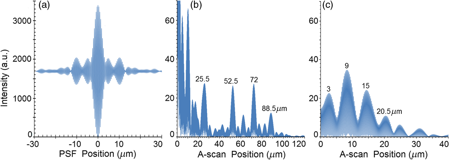 Comparing Fig. 20(b) with Fig. 20(c) clearly shows the collapse of the SDRLs toward the expected SLD axial resolution for the FSI-subtracted A-scan. Due to the significant extent of the numerous satellite pairs in the PSF [Fig. 20(a)] clearly evident between stratum peaks in the A-scan [Fig. 20(b)], the SDRLs for the A-scan do not reduce immediately from the top stratum, but first increase and then decrease for the lower strata. Is this SLD appropriate for OCT dermal application? Even though after subtracting the FSI from the A-scan, each SDRL falls within their normal stratum depth range, this SLD may also generate B-scan malignant dysplastic epithelial false positives, due to the individual SDRLs falling toward the top of the normal depth range for the stratum granulosum and stratum germinatum, as was the case for the optimally driven multiple QW SLD [Figs. 14, 10(b) and 10(d)]. The stratum’s normal depth range could be less than the SDRL for that stratum, though still in the normal depth range. Ideally, the SLD’s SDRLs should fall below the normal depth range for each stratum, as indicated in Fig. 10. Even though the T-840s’17 total bandwidth of 111 nm [Fig. 7(a)] was less than the quad-SLDs6 [145 nm in Fig. 6(b)], because the resolution limit decreases directly with the square of the central wavelength and inversely with the bandwidth [Eq. (1)], the T-840 resolution limit was seen to improve above that of the Wang Quad-SLD. A disadvantage of the T-840 is that its illumination, being of a shorter wavelength, can penetrate into the sample proportionately less than the Wang Quad SLD (Fig. 19), though this is not apparent for the depth scale of the virtual epithelial sample used. The Wang et al. Quad SLD6 has less relative SDRL inflation above its expected resolution (Table 3) compared to the T-840, because the Quad SLD PSF has only two satellite peaks that extend outward 33% less [Fig. 19(a)] than the six pairs of satellite peaks for the T-840 [Fig. 20(a)]. The reason for this is that the T-840 has four peaks, one peak more than the Quad SLD and two peaks extend below 50% of the maximum spectral intensity [Fig. 7(a)]. The resulting spread of T-840 interfering satellite peaks for each of the stratum interface full-phase PSFs, especially the FSI, restricts any thinner sample layer definition from being resolved in each A-scan, with [Fig. 20(c)] and without [Fig. 20(b)] FSI subtraction. Finally, the tandem SLD used next is presented by Andreeva et al.4 Here, the SDRLs for the highest resolution SLD, the Q-9404 [Figs. 7(b) and 21], were compared with the previous two tandem SLDs and to that of a simulated Gaussian equivalent of the Q-940 [Figs. 7(c) and 22]. That is, the simulated Gaussian spectral SLD had the same expected coherence length (1.3 μm), central wavelength (940 nm), and bandwidth (307.5 nm) as the Q-940, but instead was perfectly Gaussian [Fig. 7(c)]. Initially, the spectral and A-scan SDRL characteristics of the Q-940 are presented, and the results are compared to the previous SLDs. Fig. 21Quad-SLD Broadlighter Q-9404 with . (a) SLD full-phase PSF, , (b) A-scan, and (c) FSI-subtracted A-scan, of SDRL sample.  Fig. 22Gaussian equivalent of Quad-SLD Q-9404, in Figs. 7(b) and 7(c), with . (a) SLD full-phase PSF, , (b) A-scan, and (c) FSI-subtracted A-scan, of minimum SDRL sample.  Andeeva et al.4 reported on the Superlum Broadlighter Quadruple-SLD, the Q-940, having a demonstrated 307-nm bandwidth [Fig. 7(b)]. The average SDRL, with and without FSI subtraction, was and , respectively. This was a reduction of and an inflation of , respectively, above the expected 1.75-μm PSF FWHM resolution (Table 3). Clearly, satellite size, number, and lateral extent dominate the resolution outcome of this SLD as indicated by the interfering effect of the satellites, predicted by the PSF satellite distribution [Fig. 21(a)] and clearly showing in the A-scan itself [Fig. 21(b)]. These interfering satellite peaks inflate the SDRLs across the strata for the A-scan itself. With the FSI subtracted from the A-scan, the SDRLs collapse to unity with the expected resolution limit (Table 3). The Q-940 and the T-840 had the most inflated resolution limits of all the SLDs considered in this paper. Like the T-840 PSF, the Q-940 PSF extends out at least 25 μm [Fig. 21(a)]. The reason for this is the eight interdigitated spikes in the spectra [Fig. 7(b)], which contributed to the three primary, three secondary, and numerous smaller tertiary satellite peaks in the PSF [Fig. 21(a)]. This restricted any thinner sample layer definition in the A-scan, with and without FSI subtraction. This satellite infrastructure can be clearly seen expressing between each stratum peak, especially between the FSI and the adjacent lower top stratum [Fig. 21(b)]. However, since the spectral troughs did not extend below 50% of the maximum spectral intensity, unlike the T-840 spectrum [Fig. 7(a)], the satellite peaks were much less intense and less extended [Figs. 21(a) and 21(b)] than the T-840 [Figs. 20(a) and 20(b)]. This resulted in the average Q-940 A-scan SDRL being similarly inflated above the expected resolution (Table 3), as was the case for the Wang et al. Quad SLD, , but significantly less inflated than the T-840, . Is this SLD appropriate for OCT dermal application? If the FSI was not subtracted from the A-scan, the average SDRL, , falls toward the top of the normal depth range for the stratum granulosum and stratum germinatum, as was the case for the multiple QW SLD driven optimally [Figs. 14, 10(b) and 10(d)]. This could produce false B-scan malignant dysplastic epithelial false positives if the actual stratum depth (3 to 7 μm) fell below either of these SDRLs. Ideally, the SLD’s SDRLs should fall below the normal depth range for each stratum as indicated in Fig. 10. However, if the FSI was subtracted from the A-scan, then this SLD, Q-940, would be suitable for differentiating normal epithelial strata from swollen hyperplastic malignant epithelial strata; even the lowest stratum, the germinal stratum germinatum, could be resolved. This is because the FSI-subtracted A-scan SDRL falls below this stratum’s normal thickness. 5.9.Gaussian Equivalent of the Q-940 Quad-SLDComparing this virtual Gaussian SLD with the Q-940, one can immediately note the lack of satellite peaks [Fig. 22(a)] as predicted previously7 for the Gaussian spectral SLD with its SDRLs not significantly different from the coherence length [Table 3 and Fig. 22(b)].4 However, as is typical of the other SLD A-scans (Table 3), the lowest stratum is most difficult to determine, as it has the least reflection intensity, since it is the farthest stratum from the incident illumination [Fig. 22(b)]. Also, unexpectedly, the high intensity of the FSI does inflate the SDRL for the adjacent lower stratum. This inflated SDRL collapses upon FSI subtraction, resulting in the SDRLs’ equivalence with the expected resolution limit. There should not be any discrepancy between the and the expected resolution, PSF FWHM, for a Gaussian spectral source. However, it is not clear why the coherence length is 28% below the expected resolution, the PSF’s FWHM, as for this Gaussian source they should be equivalent. 5.10.SDRL Average SummaryTable 4 summarizes the averages of the four SDRLs, (a) to (d) in Table 3 and generates a proportion, comparing each SLD average SDRL with their PSF FWHM, the expected resolution. The absolute uncertainty is generated from each mean’s relative error. Figure 23 graphically compares the ranges for the average SDRLs of the A-scan, with and without FSI subtraction. Figure 24 compares the average SDRLs relative to the expected resolution for each SLD A-scan, with and without FSI subtraction, relative to the expected resolution, which is the SLD’s PSF FWHM. Fig. 23Table 4 summarized graphically: a comparison of the average stratum depth resolution limit for each SLD A-scan, with and without FSI subtraction. This includes the SLDs’ 95% confidence intervals, by SLD type: 5.2, 5.3,…, 5.9 referring to the SLD numbering in Table 4 above.  Fig. 24Table 4 summarized graphically: a comparison of the average SDRLs for each SLD A-scan, with and without FSI subtraction, relative to the expected resolution, which is the SLD’s PSF FWHM. 95% confidence intervals are included for each SLD type. 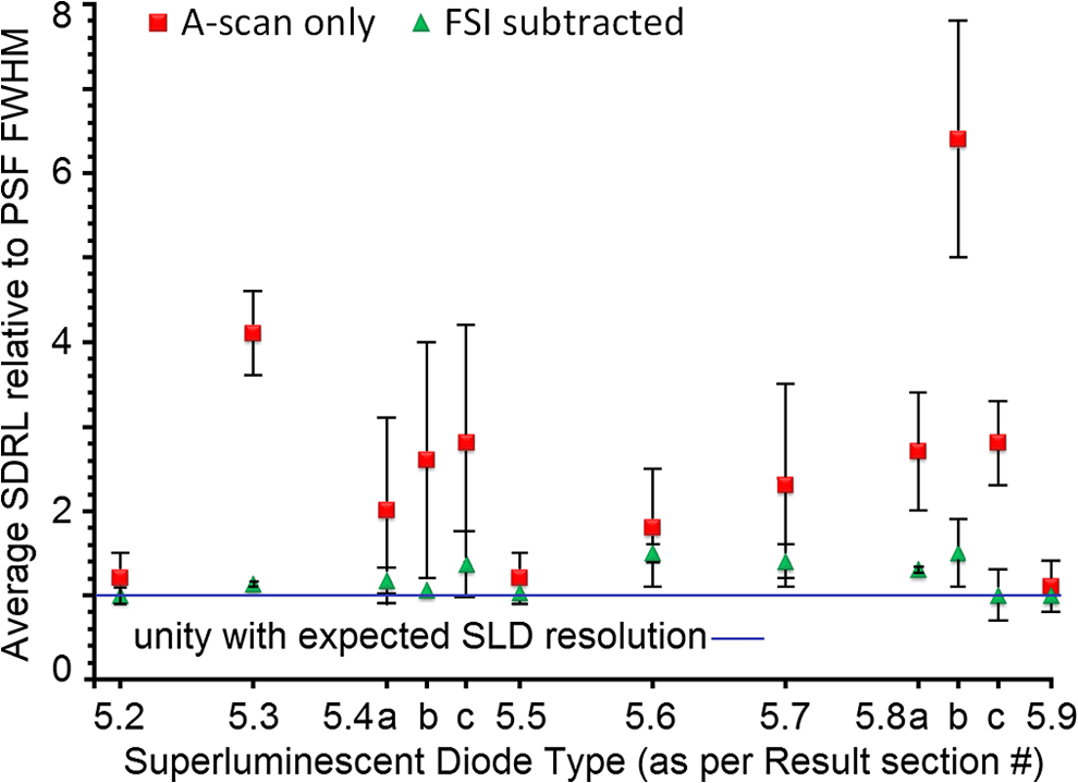 Figure 23 demonstrates the previous summary paragraph. For the SLDs with many more satellite peaks in their PSF and being far from spectrally Gaussian, there is significant improvement of the average SDRL and less variation of the SDRL between strata when their FSI is subtracted from their A-scan. If one compares the drop in the average SDRL for 5.2, 5.7a, 5.7b, and 5.7c in Table 4, these show significantly more vertical movement than for the other SLDs. Furthermore, their 95% confidence intervals are significantly less extended than the other SLDs, indicating a more stable SDRL response between strata for these SLDs, but only after FSI subtraction. Last, Fig. 24 clearly shows the benefit of FSI subtraction from the A-scan of samples like skin that have a significant surface reflection compared to strata sufficiently below the surface down to which the FSI extends. All SLDs, except three, have their A-scan average SDRL significantly different to their expected resolutions. Of these three, two are Gaussian, the bulk SLD (5.2) and the Q-940 Gaussian equivalent (5.9), and the other is significantly Gaussian, the single QD SLD (5.5). When the FSI is subtracted from each SLD A-scan, only four SLDs have their FSI-subtracted A-scan average SDRL significantly different from their expected resolutions. The multiple QD SLD (5.6) and the Q-dash SLD (5.7) have their 95% confidence interval lower limit 40% and 20% above their expected resolution limits, respectively. The other two are the Quad SLD6 (5.8a) and the T-840 SLD17 (5.8b), which have the lower limit of their 95% confidence interval 26% and 10% above their expected resolution limits, respectively. In summary, the inflation of the SDRLs above the expected resolution, noted in all real SLD examples, was both a product of the extent of the dual satellite peaks in the PSF and the reflection and depth profile of the sample. The higher the interface reflection, the greater the satellite peak intensity and the greater the adjacent strata SDRLs, especially obvious for the strata adjacent to the FSI. This is evident in all figures demonstrating satellite peaks in their A-scans [(b) and (c) in Figs. 11 to 22], as well as being indicated by the general decrease in SDRL from the top to the bottom stratum. The SLDs expressing less number and intensity of satellite peaks the quicker, by stratum, the SDRLs collapsed toward the expected SLD resolution and to the SDRLs of the FSI-subtracted A-scan. This is seen for the bulk SLD (Fig. 11), the multiple QW SLDs (Figs. 13–15), the Q-dot SLDs (Figs. 16 and 17), and the Q-dash SLD (Fig. 18), which all had a low number and intensity of satellite peaks. By contrast, the SQW SLD (Fig. 12), and the tandem SLDs, including the Quad SLD (Fig. 19), the T-840 (Fig. 20) and Q-940 (Fig. 21), all exhibited inflation, and slow decrease of their SDRLs from the top to the bottom stratum. Thus, the improvement in the SDRLs once the FSI had been subtracted from the A-scan was most evident for the later SLDs, with the greater spectral peak depths and number, and greater satellite extent in their PSFs. 5.11.Implications and ApplicationsThe choice of a SLD source for OCT dermatography depends on the stratum depth resolution needed for the particular stage of a dermal malignancy. It will also depend on the depth and optical properties of the malignant regions—birefringence, refraction, absorption, scattering, and anisotropy—compared to normal tissues, for the OCT light source (e.g., SLD) wavelength span. Implications and application of the results of this research follow. Blatter et al.28 used an extended focus swept source OCT for dermography. Their source was a Fourier-domain mode locked (FDML) laser “centered at 1310 nm with a 140-nm full bandwidth, giving an axial resolution of 12 μm in air.”28 As expected from the indications of this present research, full epidermal strata contrast were not possible, as some strata thicknesses are less than 5 μm. However, for imaging skin lesions, their FDML laser resolution and penetration were sufficient and necessary, respectively. Gladkova et al.29 concluded that even using an SLD with a coherence length resolution of 16 μm, OCT can distinguish general pathological reactions such as active inflammation and necrosis as well as distinguishing hyperkeratosis, parakeratosis, and intradermal cavities. However, such noninvasive optical biopsy imaging modalities as OCT would be useful, if possible, to assist in detecting premalignant dermatopathologies. Confirming the advantage of higher resolution OCT sources, Korde et al.30 concluded that the use of such sources significantly reduced false positives for their dermal malignancy, implied by this present research. However, it is also the OCT source PSF structure—satellite peak, number, size, and extent—that affects resolution, as indicated by the present results. Korde et al. used an “amplified fiber source” not an SLD, which typically have even less Gaussian-like spectra than SLDs. A recent review of optical techniques for detecting skin cancer31 concluded that, although successful in showing deep margins of skin tumors and inflammatory skin diseases, OCT could not distinguish early skin disease stages. However, all their stated OCT examples used sources with axial resolution in tissue exceeding 8 μm, clearly not able to contrast normal from premalignant epithelium due to the thinness of some epithelial strata. The exception was the high definition OCT, which did provide “valuable extra diagnostic information.”31 The present SLD research has clearly shown that it is not just the coherence length that determines image resolution and contrast. The SLD PSF’s shape and the tissue’s morphology and optical parameters together determine the degree of image contrast and resolution required for early-stage detection of dermal pathology. The application of the above SLD characterization to a particular dermal pathology can be considered. Melanoma can present as a dermal malignancy, expressing as hyperplastic melanocytes in the germinal basal layer. They form small dysplastic nodules there, causing this layer to thicken significantly [Fig. 9(b)]. As the melanoma cells are significantly distended (accelerated melanogenesis) and necrotic in the nodules [Fig. 9(b)], the density of nuclei and intracellular organells and products may be significantly less, per unit volume, than the surrounding squamous cells and normal melanocytes of the germinal stratum [Fig. 9(b)]. As such, the average refractive index of the nodules should be closer to that of water and less than the surrounding normal epidermal and dermal cells. Because water’s refractive index is wavelength dependent, for the total wavelength span of all the SLDs in Table 5 (770 to 1610 nm), the total refractive index span is 1.330 to 1.317 (Table 5). This span is less than the refractive index of the surrounding epidermal and dermal strata (Table 1). Depending on the range of absorption coefficients for each SLD’s wavelength (Table 5), for these malignant nodules (Fig. 10), the longer wavelength SLD () will have a greater refractive index contrast than the surrounding strata but more water absorption, while it will be vice versa for shorter wavelength () SLDs. This trade-off is also apparent for resolution and penetration depth; for a given bandwidth, the shorter the wavelength, the better the resolution but the lower the penetration depth.7 Table 5Water’s refractive index32 and absorption coefficient33 ranges for each SLD.
Continuing with the example of which SLD type would best suit premelanoma differentiation, only the Q-940 demonstrated SDRLs less than the normal depth range for all epithelial strata. It has a wavelength span that shows a water refraction close to 1.33 (Table 5) and relatively minimal water absorption (Table 5: 0.024 to 0.52) compared to the other SLDs. If the surrounding epithelial strata refractive index extends upward from for the stratum germinatum to for the stratum spinosum (Table 1), then, including the fact of minimal water absorption, the optical contrast between the melanoma nodule and the surrounding normal epidermis and reticular dermis should be evident using this SLD. Given their degree of resolution limit and the water-tissue optical contrast, the Q-940 could be useful for contrasting normal and premalignant hyperplastic dermal strata using OCT. Also, given this degree of resolution for the Q-940, depending on sufficient normal pathological tissue optical contrast as well as a suitable depth of the pathological region, other dermal pathologies may be differentially imaged using the Q-940 SLD for OCT imaging. One is cautioned to consider, among other factors, that:
However, what can be concluded is the comparative relativity of the resolution (SDRL) performance of the different SLD sources in a TD OCT system applied to a constant realistic refractive index 1-D epidermal cross-section, as identified from the dermatological literature (Tables 1 and 2). The advantage of this OCT simulator is evidenced by the ability to visualize the expected autocorrelated PSF and the cross-correlation function, the tissue model A-scan, from a digitized real OCT source spectrum. The versatility that this imparts to the characterization of real OCT systems is evidenced by 6.Future DirectionsAt this stage in the model’s extrinsic evolution, it is important to clarify further what this model assumes, as eluded to above. Future models will address these issues. The model assumes:
The potential to use the model to study other real OCT light sources including solid state lasers, super-continuum sources, and black body radiation sources, as well as ODLs and sample structures, can better characterize the functionality of OCT components and systems. Future work will utilize the model to interferometrically characterize these OCT components to improve understanding of the effects these OCT elements have on the resulting A-scan, with implications for 2-D B-scans and 3-D C-scans. The model will be made more realistic by including a Kubelka-Munk-theory model adaptation.26,34 This will allow more specific tissue parameters to be defined, including scattering, absorption, and anisotropy coefficients. With this OCT-model adaptation, greater similarity to real tissue A-scans is envisaged. 7.ConclusionUsing an improved LCI model, we have shown a comparison of real broadband SLD light sources used for OCT. The model was able to digitize real OCT source spectral data and produce the corresponding PSF and A-scan of a simplified human epidermal tissue phantom. This enabled the identification of satellite peak size, number, and extent, allowing the prediction and demonstration of the actual resolution inflation beyond that expected: the coherence length. Both the PSF and A-scan results confirmed previous research7 that used simulated virtual multi-Gaussian light sources: i.e., the actual resolution inflation above that expected was proportional to the number and depths of the peaks in the source spectrum. The closer the source spectrum to a Gaussian spectrum, the closer the A-scan resolution to the expected coherence length. The study indicates that care must be taken when choosing a light source for OCT imaging, as increases in the SLD spectral bandwidth do not necessarily translate to improvements in axial resolution. ReferencesA. F. Fercher,
“Optical coherence tomography,”
J. Biomed. Opt., 1
(2), 157
–173
(1996). http://dx.doi.org/10.1117/12.231361 JBOPFO 1083-3668 Google Scholar
J. A. Izattet al.,
“Optical coherence tomography for biodiagnostics,”
Opt. Photon. News, 8
(5), 41
–47
(1997). http://dx.doi.org/10.1364/OPN.8.5.000041 OPPHEL 1047-6938 Google Scholar
W. Drexleret al.,
“Ultrahigh resolution optical coherence tomography,”
Optical Coherence Tomography: Technology and Applications, 239
–280 Springer-Verlag, Berlin, EU
(2008). Google Scholar
E. V. Andreevaet al.,
“Novel superluminescent diodes and SLD-based light sources for optical coherence tomography,”
Proc. SPIE, 6627 662703
(2007). http://dx.doi.org/10.1117/12.724174 PSISDG 0277-786X Google Scholar
L. H. Liet al.,
“Wide emission spectrum from superluminescent diodes with chirped quantum dot multilayers,”
Electron. Lett., 41
(1), 41
–42
(2005). http://dx.doi.org/10.1049/el:20056995 ELLEAK 0013-5194 Google Scholar
H. WangM. W. JenkinsA. M. Rollins,
“A combined multiple-SLED broadband light source at 1300 nm for high resolution optical coherence tomography,”
Opt. Commun., 281
(7), 1896
–1900
(2008). http://dx.doi.org/10.1016/j.optcom.2007.08.073 OPCOB8 0030-4018 Google Scholar
P. V. Janszet al.,
“Modelling of low coherence interferometry using broadband multi-Gaussian light sources,”
Photon. Sensors, 2
(3), 247
–258
(2012). http://dx.doi.org/10.1007/s13320-012-0069-0 1674-9251 Google Scholar
P. V. Janszet al.,
“Simulation of optical delay lines for optical coherence tomography,”
in Proc. Quantum Electronics Conf. & Lasers and Electro‐Optics (CLEO/IQEC/PACIFIC RIM),
1400
–1402
(2011). Google Scholar
P. V. JanszG. WildS. Hinckley,
“A micro‐photonic stationary optical delay line for fibre optic TD OCT,”
in Proc. Opto‐Electronics and Communications Conf. and the Australian Conf. on Optical Fibre Technology (OECC/ACOFT),
(2008). Google Scholar
M. Friebelet al.,
“Influence of oxygen saturation on the optical scattering properties of human red blood cells in the spectral range 250 to 2000 nm,”
J. Biomed. Opt., 14
(3), 034001
(2009). http://dx.doi.org/10.1117/1.3127200 JBOPFO 1083-3668 Google Scholar
V. R. Shidlovski,
“Superluminescent diode light sources for OCT,”
Optical Coherence Tomography: Technology and Applications, 281
–299 Springer-Verlag, Berlin, EU
(2008). Google Scholar
S. G. Adie,
“Enhancement of Contrast in Optical Coherence Tomography: New Modes, Methods and Technologies,”
Univ. of Western Australia, Perth,
(2007). Google Scholar
D. Huanget al.,
“Optical coherence tomography,”
Science, 254
(5035), 1178
–1181
(1991). http://dx.doi.org/10.1126/science.1957169 SCIEAS 0036-8075 Google Scholar
J. WangM. J. HampD. T. Cassidy,
“Design considerations for asymmetric multiple quantum well broad spectral width superluminescent diodes,”
IEEE J. Quantum Electron., 44
(12), 1256
–1262
(2008). http://dx.doi.org/10.1109/JQE.2008.2003104 IEJQA7 0018-9197 Google Scholar
A. Somerset al.,
“Optical gain properties of InAs/InAlGaAs/InP quantum dash structures with a spectral gain bandwidth of more than 300 nm,”
Appl. Phys. Lett., 89
(6), 061107
(2006). http://dx.doi.org/10.1063/1.2266994 APPLAB 0003-6951 Google Scholar
B. S. Ooiet al.,
“Quantum dashes on InP substrate for broadband emitter applications,”
IEEE J. Sel. Top. Quantum Electron., 14
(4), 1230
–1238
(2008). http://dx.doi.org/10.1109/JSTQE.2008.919277 IJSQEN 1077-260X Google Scholar
B. Censeet al.,
“Volumetric retinal imaging with ultrahigh-resolution spectral-domain optical coherence tomography and adaptive optics using two broadband light sources,”
Opt. Express, 17
(5), 4095
–4111
(2009). http://dx.doi.org/10.1364/OE.17.004095 OPEXFF 1094-4087 Google Scholar
G. T. Tearneyet al.,
“Determination of the refractive index of highly scattering human tissue by OCT,”
Opt. Lett., 20
(21), 2258
–2260
(1995). http://dx.doi.org/10.1364/OL.20.002258 OPLEDP 0146-9592 Google Scholar
Realistic Skin Model (RSM)—BIO Toolkit Interactive Script for ASAP,
(2008). Google Scholar
T. IgarashiK. NishinoS. K. Nayar,
“The appearance of human skin,”
(2005). Google Scholar
A. KnüttelM. Boehlau-Godan,
“Spatially confined and temporally resolved refractive index and scattering evaluation in human skin performed with optical coherence tomography,”
J. Biomed. Opt., 5
(1), 83
–92
(2000). http://dx.doi.org/10.1117/1.429972 JBOPFO 1083-3668 Google Scholar
B. Formanet al.,
“Is superficial spreading melanoma still the most common form of malignant melanoma?,”
J. Am. Acad. Dermatol., 58
(6), 1013
–1020
(2008). http://dx.doi.org/10.1016/j.jaad.2007.10.650 JAADDB 0190-9622 Google Scholar
S. Hatai,
“The refractive index of the blood serum of the albino rat at different ages,”
J. Biol. Chem., 35
(3), 527
–552
(1918). JBCHA3 0021-9258 Google Scholar
D. K. SardarL. B. Levy,
“The optical properties of whole blood,”
Lasers Med. Sci., 13
(2), 106
–111
(1998). http://dx.doi.org/10.1007/s101030050062 LMSCEZ 1435-604X Google Scholar
H. LiL. LinS. Xie,
“Refractive index of whole blood with different types in the visible and NIR ranges,”
Proc. SPIE, 3914 517
–521
(2000). http://dx.doi.org/10.1117/12.388073 PSISDG 0277-786X Google Scholar
M. J. C. Van Gemertet al.,
“Skin optics,”
IEEE Trans. Biomed. Eng., 36
(12), 1146
–1154
(1989). http://dx.doi.org/10.1109/10.42108 IEBEAX 0018-9294 Google Scholar
H. Dinget al.,
“Refractive indices of human skin tissues at eight wavelengths and estimated dispersion relations between 300 and 1600 nm,”
Phys. Med. Biol., 51
(6), 1479
–1489
(2006). http://dx.doi.org/10.1088/0031-9155/51/6/008 PHMBA7 0031-9155 Google Scholar
C. Blatteret al.,
“In situ structural and microangiographic assessment of human skin lesions with high-speed OCT,”
Biomed. Opt. Express, 3
(10), 2636
–2646
(2012). http://dx.doi.org/10.1364/BOE.3.002636 BOEICL 2156-7085 Google Scholar
N. D. Gladkovaet al.,
“In vivo optical coherence tomography imaging of human skin: norm and pathology,”
Skin Res. Technol., 6
(1), 6
–16
(2000). http://dx.doi.org/10.1034/j.1600-0846.2000.006001006.x 0909-752X Google Scholar
V. R. Kordeet al.,
“Using coherence tomography to evaluate skin sun damage and precancer,”
Lasers Surg. Med., 39
(9), 687
–695
(2007). http://dx.doi.org/10.1002/(ISSN)1096-9101 LSMEDI 0196-8092 Google Scholar
M. A. Calinet al.,
“Optical techniques for the noninvasive diagnosis of skin cancer,”
J. Cancer Res. Clin. Oncol., 139
(7), 1083
–1104
(2013). http://dx.doi.org/10.1007/s00432-013-1423-3 JCROD7 1432-1335 Google Scholar
N. Polyanskiy,
“Refractive index database,”
(2013) http://refractiveindex.info/legacy/?group=LIQUIDS&material=Water May ). 2013). Google Scholar
G. M. HaleM. R. Querry,
“Optical constants of water in the 200-nm to 200-μm wavelength region,”
Appl. Opt., 12
(3), 555
–563
(1973). http://dx.doi.org/10.1364/AO.12.000555 APOPAI 0003-6935 Google Scholar
R. R. AndersonJ. A. Parrish,
“The optics of human skin,”
J. Investig. Dermatol., 77
(1), 13
–19
(1981). http://dx.doi.org/10.1111/jid.1981.77.issue-1 JIDEAE 0022-202X Google Scholar
BiographyPaul Vernon Jansz is a PhD candidate at Edith Cowan University (ECU). He received his BSc in physical science and mathematics, and first class honors in physics from ECU in 1998 and 2003, respectively. He is the author of 30 refereed publications. His current research interests include low coherence interferometry imaging and improving light-sensing pixel resolution, achieving crosstalk free pixels. He is a member of SPIE, OSA, and ACS. Steven Richardson is a senior lecturer in mathematics in the School of Engineering at Edith Cowan University. He received his BSc in mathematics with first class honors (summa cum laude) in 2002, and his PhD in “Numerical Methods for Solving Optimal Feedback Control Problems” in 2007, both from the University of Western Australia. He has published seven journal articles, nine conference papers, and a book chapter. Graham Wild is senior lecturer in aerospace and aviation, and aviation program director, at RMIT University. He received his BS degree in physics and mathematics, with first class honors in physics and PhD in engineering from ECU in 2005 and 2010, respectively. He also received a MS in photonics and optoelectronics from the University of New South Wales in 2008. He is a member of SPIE, the IEEE, and the Royal Aeronautical Society. Steven Hinckley is an associate professor in the School of Engineering at ECU. He received his BSc with honors in physics and his PhD in physics from the University of New South Wales, in 1979 and 1986, respectively. He is the author of over 100 refereed publications. He is a member of SPIE, OSA, the American Vacuum Society, and the Australian Optical Society. His research interests include biomedical imaging, thin films, photovoltaics, and optical sensing. |
|||||||||||||||||||||||||||||||||||||||||||||||||||||||||||||||||||||||||||||||||||||||||||||||||||||||||||||||||||||||||||||||||||||||||||||||||||||||||||||||||||||||||||||||||||||||||||||||||||||||||||||||||||||||||||||||||||||||||||||||||||||||||||||||||||||||||||||||||||||||||||||||||||||||||||||||||||||||||||||||||||||||||||||||||||||||||||||||||||||||||||||||||||||||||||||||||||||||||||||||||||||||||||||||||||||||||||||||||||||||||||