User-guided segmentation for volumetric retinal optical coherence tomography images

Xin Yin; Jennifer R. Chao; Ruikang K. Wang

doi:10.1117/1.JBO.19.8.086020

22 August 2014 User-guided segmentation for volumetric retinal optical coherence tomography images

Xin Yin, Jennifer R. Chao, Ruikang K. Wang

Author Affiliations +

Journal of Biomedical Optics, Vol. 19, Issue 8, 086020 (August 2014). https://doi.org/10.1117/1.JBO.19.8.086020

Abstract

Despite the existence of automatic segmentation techniques, trained graders still rely on manual segmentation to provide retinal layers and features from clinical optical coherence tomography (OCT) images for accurate measurements. To bridge the gap between this time-consuming need of manual segmentation and currently available automatic segmentation techniques, this paper proposes a user-guided segmentation method to perform the segmentation of retinal layers and features in OCT images. With this method, by interactively navigating three-dimensional (3-D) OCT images, the user first manually defines user-defined (or sketched) lines at regions where the retinal layers appear very irregular for which the automatic segmentation method often fails to provide satisfactory results. The algorithm is then guided by these sketched lines to trace the entire 3-D retinal layer and anatomical features by the use of novel layer and edge detectors that are based on robust likelihood estimation. The layer and edge boundaries are finally obtained to achieve segmentation. Segmentation of retinal layers in mouse and human OCT images demonstrates the reliability and efficiency of the proposed user-guided segmentation method.

1. Introduction

Optical coherence tomography (OCT) is a noninvasive imaging technology that is capable of capturing micrometer-resolution three-dimensional (3-D) images of optical scattering media, including biological tissue.¹^,² It is now widely used as a research and clinical tool for the investigation of retinal diseases in both humans and animal models.³^–⁷ The measurement of geometrical dimensions (i.e., biometry) of physiological and pathological retinal layers and features is one of the primary functions of OCT imaging. Images of changes in layered retinal structures aid in the diagnosis, treatment, and management of many blinding diseases.⁸^–¹⁰ In this regard, the algorithms for correctly segmenting the retinal layers or features play an important role. However, OCT images, particularly those acquired from patients and animal models with eye disease, are sometimes of low contrast (i.e., noisy) and have irregular features. For these simple reasons, it remains a challenging task to achieve satisfactory segmentation of the retinal layers in OCT images using automated segmentation techniques.

The retina is composed of distinct physiological layers, including the nerve fiber layer (NFL), ganglion cell layer (GCL), inner plexiform layer (IPL), outer plexiform layer (OPL), external limiting membrane (ELM), and inner/outer segments (IS/OS). Because the different cell compositions of each layer have distinct optical scattering properties, these layered tissues usually appear as varied intensities in the OCT images with a signal transition from one layer to another which appears as boundary line (interface) (see Fig. 1). It should be pointed out that the boundary between the GCL and IPL in human eye appears weak. The GCL in mouse eye is thin, which is sometimes difficult for OCT to resolve. Therefore, most segmentation studies treat the GCL and IPL as one layer, giving the NFL, GCL+IPL, OPL, ELM, and IS/OS layers in the segmentation.¹¹^–²⁷ Over the last decade, various segmentation techniques were developed to segment the images from one-dimensional to 3-D based on algorithms from simple intensity threshold to complex machine learning algorithms.¹¹^,¹² The majority of these segmentation algorithms are based on analyzing the variations of OCT signal intensities along the A-scans (depth scan) or in two-dimensional (2-D) cross-sectional images (B-scan).¹³^–¹⁵ It is possible to achieve fast segmentation based on this gradient information;¹⁶ however, these algorithms are prone to errors when detecting abnormal edge information or images that appear noisy. To reduce the erroneous edge and layer detection when the image appears noisy (either globally or locally), two approaches have been proposed. One is to improve the robustness of the algorithms to detect the edges or layers.¹⁷^,¹⁸ Another approach is to connect the individual edge detectors together using a 2-D curve or 3-D mesh.¹⁹^,²⁰ By analyzing the information presented in the neighborhood, such as curvature, or applying a global optimization algorithm, the resulting boundaries of the retinal layers become sufficiently smooth and the chance of erroneous edge detection is reduced.²¹ Usually, the parameters of the edge detection algorithms are assigned empirically or are trained through the use of other manually segmented subsets.¹⁷^,¹⁸^,²² To achieve high accuracy in the quantification of geometrical dimensions (e.g., thickness) of retinal layers, two-step strategies, in which different algorithms are utilized in each step, are often utilized to perform segmentation.²³ The key to the success of segmenting retinal layers is to correctly detect the layers or their boundary edges in the OCT images. Most previously proposed segmentation techniques can meet this goal when it is treated as a local optimization problem. It is still a challenging task to achieve global optimization.

Fig. 1

Typical optical coherence tomography (OCT) B-scan of retina in a mouse eye and the assignment of physiological layers and features. Scale bar: $100 μ m$ .

Despite the fact that a number of prior robust algorithms that are capable of achieving high-level automatic segmentation have been reported,²²^–²⁷ many clinical practices still continue to use manual segmentation as the technique of choice for OCT image segmentation. Reluctance to accept the fully automatic approach may be due to the concerns about its insufficient reliability in cases where the target layers and features may differ from the norm and because of insufficient accuracy in delineating the desired physiological and pathological features in a noisy background.

A similar situation occurs in the arena of medical imaging, including magnetic resonance imaging (MRI). In order to increase the reliability and confidence of feature segmentation in MRI, there has been increased interest in developing user-guided segmentation instead of fully automated algorithms.²⁸^,²⁹ The advantage of user-guided segmentation algorithms is that they have the potential to efficiently combine the features of human and computer to achieve the segmentation of medical images. Humans are remarkably sensitive and accurate in recognizing tissue patterns to achieve global optimization, while the computer can achieve local optimization with high speed. The user-guided segmentation system can, therefore, be reliable and efficient. In the system, a user typically assigns some key features such as points or curves, and then the computer finishes the rest of the segmentation task in delineating or searching for the tissue of interest guided by the user-defined key features. Determining how to assign and interpolate the key features and how to trace entire layers based on these key features are the main tasks in designing user-guided segmentation algorithms.

In this paper, a user-guided algorithm is proposed and designed for the segmentation of retinal layers in OCT images that were acquired using a custom-built OCT system reported in Refs. 30 31.32.33.34. to 35. The user-guided algorithm, the double line model (DLM) (described in detail in Sec. 2.2), is based on a 2-D robust layer and edge detectors, and was used to extract the shapes of an embryo heart for analyzing heart development.³⁶^–³⁸ DLM detects local layer patterns and edges in places where the images appear noisy or distorted due to pathological reasons. However, DLM does not work well in terms of global optimization problems; for example, it often fails to trace the layered structures at regions with irregularly layered structures and/or with low contrast and holes within the retinal layers. To mitigate this problem, we propose that before the algorithm begins to work on the 3-D dataset, a user first delineates a number of user-defined sketch lines on irregular or otherwise difficult features to correctly guide the DLM in tracing the retinal layers. The proposed user-guided segmentation method is reliable and can segment noisy and irregular OCT images of the retina.

2. Method

In this section, a 3-D OCT image of the posterior segment of the mouse eye is used as an example to illustrate the application of the user-guided segmentation algorithm. Because it is difficult for DLM to deal with a layer whose thickness is thinner than 3 pixels, as a preprocessing step we select an appropriate scale to adjust the OCT image size in the depth direction so that the thinnest target layer is thicker than 3 pixels.

The steps of the user-guided segmentation of retinal layers are shown in Fig. 2. The segmentation process starts with assigning user-defined lines for retinal layers and features where the image appears irregular or abnormal [see Figs. 2(a) and 2(b)]. Then, a two-step segmentation strategy follows: (1) tracing the retinal layers to obtain approximate locations of the layers and boundaries [see Figs. 2(b) to 2(d)] and (2) obtaining the accurate boundaries of the retinal layers [see Figs. 2(e) to 2(f)]. In the following subsections, segmentation of the retinal layers is illustrated in detail.

Fig. 2

Segmentation steps of retinal layers. (a) Sketch of an example three-dimensional (3-D) retinal image. In places where the image appears irregular, conventional automated segmentation methods often fail to achieve segmentation. (b) User assigns static and adaptive lines at the irregular features. (c) Using the layer double line models (DLMs) on the adaptive line to detect and trace entire layers. (d) The segmentation result after layer tracing. (e) Using the edge-DLM on the boundary of the layers to detect the local edges. (f) Final segmentation result.

2.1.

Assigning the User-Defined Lines

The first step of segmentation is to assign a number of user-defined lines in the 3-D OCT images [see Figs. 2(b) and 3]. To assign the user-defined lines, an interactive interface is developed for users to navigate the 3-D OCT images frame by frame. The XYZ coordination is defined as shown in Fig. 3: the $X$ axis is the abscissa of the B-scan image, the $Y$ axis is the sequence number of the image, and the $Z$ axis is the ordinate of the B-scan image (depth). The user selects a 2-D B-frame (cross-sectional image) that may be at any location within the 3-D image and then rotates the image around its local $Z$ axis by using a computer mouse in order to observe anatomical features appearing within it. On the computer screen, the user-defined lines are then assigned in the cross-sectional image.

Fig. 3

Assigning user-defined lines to the OCT images. (a) Adaptive lines with DLMs. Static lines are assigned at places where the image is of (b) low contrast or (c) irregular. Scale bar: $100 μ m$ .

The user-defined lines are classified into static lines and adaptive lines. A static line is a line that does not change its attributes, such as the shape, orientation, and position, when using DLM to detect and trace the retinal layers during segmentation, i.e., it is a fixed line [see Figs. 3(b) and 3(c)]. An adaptive line is a line that is assigned to a retinal layer that would change its attributes in order to arrive at a state that optimizes its position according to the local features, i.e., it has an adaptive nature during segmentation [Fig. 3(a)]. The static lines are assigned at locations where conventional automatic segmentation methods often fail to detect layered features: (1) irregular layered structures; (2) regions with low contrast; and (3) holes in retinal layers [Figs. 3(b) and 3(c)]. The major function of the static lines is to guide layer tracing to continually trace the correct position of the retinal layers. For example, because there are no retinal-like layers at optic nerve head (ONH), the layer tracing would certainly fail in the region of ONH. Using static lines can address this issue. Thus, assigning static lines to enhance or add the layer pattern transforms the complex problem to a simple one and largely minimizes the mistakes when using DLM to trace entire retinal layers. Adaptive lines connect the DLMs together, becoming the seed layer for the algorithm to detect and trace the retinal layers in the entire 3-D dataset. They are assigned on the retinal layer in selected 2-D B-scan images [Fig. 3(a)]. When the DLMs detect the local layer and modify its attributes, the adaptive line also changes its shape and orientation according to the new position of the DLMs.

2.2.

Double Line Model

The DLMs assigned along the adaptive line are used to detect the retinal layer and edge in the 2-D sectional image [see Fig. 3(a)]. The DLM is a robust layer and edge detector that can detect local layers and edges within the 2-D image.³⁶ It is developed from the adaptive model based on the theory of robust signal detection and estimation.³⁹^,⁴⁰ It has two parallel lines that divide the surrounding region into internal and external regions (Fig. 4). By computing the likelihood between the DLM and the internal and external regions of the local image, the DLM can efficiently identify the target tissue from the surrounding tissue.

Fig. 4

Schematic of DLM. Optimizing the attributes of DLM shown in (b) to detect layer patterns or edges in an OCT image (a). The layer-DLM (c) is used to detect the layers, while the edge-DLM (d) detects edges in the OCT image.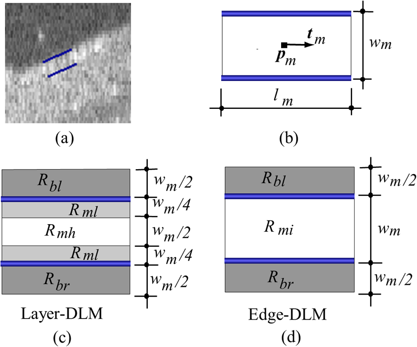

When the DLM is used to detect local layers or edges within the tissue of interest [see Fig. 4(a)], the algorithm scales, shifts, and rotates the DLM by adjusting its basic parameters, or attributes, to find its local optimized state. The basic parameters of the DLMs are width $w_{m}$ , length $l_{m}$ , position vector $p_{m}$ , and direction vector $t_{m}$ [see Fig. 4(b)]. $t_{m}$ is parallel to the lines of the DLM. Adjusting the width $w_{m}$ and length $l_{m}$ scales the DLM. Adjusting the position $p_{m}$ and direction $t_{m}$ shifts and rotates the DLM, respectively. The algorithm uses $M = {w_{m}, l_{m}, p_{m}, t_{m}}$ to present the states of the DLM.

When the DLM is used to detect retinal layers, it is designated as the layer-DLM. In OCT images, the signal strength at the interface between two layers is usually higher than that of its neighboring regions. The intensities within one retinal layer also sometimes appear different from those of other layers. Accordingly, the features of the retinal layer-DLM are divided into a high-intensity foreground region $R_{m h}$ , a low-intensity foreground region $R_{m l}$ , a right background region $R_{b r}$ , and a left background region $R_{b l}$ [see Fig. 4(c)]. The foreground regions, $I_{f h}$ and $I_{f l}$ , are estimated using the median intensity within $R_{f h}$ and $R_{f l}$ , and the background regions, $I_{b r}$ and $I_{b l}$ , are similarly estimated within $R_{b r}$ and $R_{b l}$ . When the layer-DLM matches the target layer, the intensity of the DLM would be similar to that of the foreground of the target tissue but different from the background. Thus, the likelihood $L_{l}$ between the layer-DLM at the state $M$ and the target tissue layer in a cross-sectional image is computed by

Eq. (1)

L_{l} (M | x) = \frac{1}{I_{f h}} \sum_{x \in R_{m i}} \frac{| I (x) - I_{b r} | + | I (x) - I_{b l} |}{A (R_{m i})} + \frac{1}{I_{f h}} (\sum_{x \in R_{m h}} \frac{- | I (x) - I_{f h} |}{A (R_{m h})} + \sum_{x \in R_{m l}} \frac{- | I (x) - I_{f l} |}{A (R_{m l})}),

where

I (x)

is the intensity of the pixel located at position

x

in the B-scan image and

A ()

is the area of the region that represents the sum of the pixels within the region. For example,

A (R_{m i})

is the number of pixels in the region

R_{m i}

. The first summed item computes the difference between internal region intensity and background, and the second and third summed items compute the similarity between the internal region intensity and the foreground. The local retinal layer is found by shifting, scaling, and rotating the layer-DLM to maximize

L_{l}

.

When the DLM is used to detect the edges, it is designated as the edge-DLM [see Fig. 4(d)]. The regions of the edge-DLM are internal region $R_{m i}$ , the left background region $R_{b l}$ , and the right background region $R_{b r}$ . The likelihood $L_{e}$ between the edge-DLM and the real edge in an image is computed by

Eq. (2)

L_{e} (M | x) = \frac{1}{A (R_{m i})} \sum_{x \in R_{m i}} (| I (x) - I_{b r} | + | I (x) - I_{b l} | - | I (x) - I_{f} |),

where

I_{f}

is the foreground that is the median intensity within the internal region

R_{m i}

. Other variables are the same as described in Eq. (1). The edge likelihood computes the difference between the internal region intensity and the background as well as the similarity between internal region intensities and foregrounds. Because the edge should be narrow, the width of the edge-DLM is fixed at 4 pixels. The local edge in the B-scan image is found by shifting and rotating the edge-DLM to maximize

L_{e}

.

2.3.

Tracing the Layer Using Layer-DLM

Once the user assigns a number of static lines and adaptive lines in the 3-D images [see Fig. 2(b)], the algorithm starts to trace the layers using layer-DLMs within entire 3-D images [see Fig. 2(c)]. The adaptive line is usually assigned on the first B-scan image [see Fig. 3(a)]. The layer-DLMs will start from this adaptive line. The direction of the DLM is parallel to the tangent of the adaptive line. The DLM is shifted left or right and zoomed in or out to detect the local layer position to maximize $L_{l}$ in Eq. (1). After the DLM finds the local optimized position, the adaptive line adjusts its shape and orientation according to the new positions of the layer-DLM. To reduce erroneous detection by the layer-DLM, the adaptive line is smoothed using the mean position of adjacent points.

The smoothed adaptive line is then copied to the next B-scan image as the initial adaptive line [see Fig. 2(c)]. At this next B-scan image, if there are any points that are already defined by the static lines, the adaptive line will be adjusted to the position of the point on the static line. The static line is always given priority because this is where the features within OCT images have already been identified by the user and are considered to be fixed. The DLM then works on this adaptive line in the new B-scan image to detect the local layers according to Eq. (1). The process of detecting the local layers using layer-DLM, smoothing, and copying the resulting adaptive line to the next B-scan image is repeated until the last B-scan image within the entire 3-D image is completed. The final results are then smoothed using the mean position of four adjacent points in the 3-D space. An example result is shown in Fig. 5(a), where each physiological interface is enclosed by the two lines of all DLMs.

Fig. 5

Adjusting the boundary lines of retinal layers. (a) The layer-DLM gives a suboptimal segmentation result, particularly at the noisy boundaries, e.g., nerve fiber layer (NFL). (b) The original B-scan image. (c) Preprocessed image of (b) with enhanced boundaries. (d) Accurate boundaries detected by using the edge-DLM. Scale bar: $100 μ m$ .

Upon scrutinizing Fig. 5(a), it is evident that segmentation using the layer-DLM needs some improvement, particularly in the interface boundaries that appear noisy, e.g., NFL. It is, therefore, necessary to perform an additional adjustment to the boundary lines of the segmented retinal layers. This task is performed by the edge-DLM as described below.

2.4.

Adjusting Retinal Layer Boundaries Using Edge-DLM

Certain retinal boundary lines, such as the interface between the vitreous humor and the NFL, can appear quite noisy in the original image [see Fig. 5(b)]. In order to adjust the boundary lines of the NFL, the original image is preprocessed to enhance the retinal layers. First, the intensity is smoothed using a $3 \times 3 pixel$ mean filter to reduce noise in the original image. Then, an adaptive threshold is applied to process the image. If the intensity of a pixel is stronger than the median intensity in a small local window, it is considered as the foreground and a new intensity value of 128 is assigned. Otherwise, it is considered background and assigned a value of 0. The small window size is approximately twice that of the target tissue layer as defined by the layer-DLM. Finally, the intensity is smoothed using a $3 \times 3 pixel$ mean filter to further reduce noise. This process significantly enhances the retinal layer boundary information [see Fig. 5(c)].

The edge-DLM is then used to adjust the boundary lines of the layers [see Fig. 2(e)]. After the edge-DLM detects the local edges within the preprocessed image by maximizing the edge likelihood in Eq. (2), the boundary lines are adjusted to the new positions of the edge-DLMs. All of the 2-D boundary lines form the 3-D boundary surface of the retinal layers. The final step of the segmentation is to smooth the 3-D boundaries by using the mean position of four adjacent points to reduce the error [see Fig. 5(d)].

2.5.

Thickness of the Segmented Layers

After performing segmentation of the retinal layers, it is a straightforward process to provide quantification of the thickness of the retinal layers. Most prior studies compute the thickness by using the distance between two cross-points (point $A$ and $B$ in Fig. 6) of the A-scan line and layer boundaries. However, when the A-scan line is not perpendicular to the boundary of the layer, the thickness computed using this traditional method is not accurate, because it would be thicker than the real thickness. In an effort to improve the accuracy of layer thickness quantification, we computed the thickness by considering the local normal to the surface (see Fig. 6). To compute the correct local 3-D normal to surface, the scale of the segmented layers is adjusted to the same scale in $X$ , $Y$ , $Z$ directions. Then, the local normal $N_{a}$ on the top surface and the local normal $N_{b}$ on the bottom surface are computed. Next, we compute a normal $N_{c}$ , that is, a unit vector with its direction the same as $N_{a} + N_{b}$ . The thickness $T$ is the projection of $A B$ on $N_{c}$ and is computed by $T = | A B | • N_{c}$ , which is the length of $B C$ . Finally, the thickness map is obtained by computing the thickness at all positions on the $X Y$ plane.

Fig. 6

Computing the thickness of retinal layers. Plane $T$ is the top surface of a layer and plane $S$ is the bottom surface of the layer. Line $g$ is the OCT probe-beam position, i.e., the A-scan line. The plane $R$ is the plane passing through the A-scan line $g$ and the vector $N_{c}$ that is formed between the top surface normal $N_{a}$ and the bottom surface normal $N_{b}$ .

3. Results

The segmentation algorithm was applied to 3-D datasets resulting from optical micro-angiography (OMAG) imaging of the posterior segments of eyes in both mouse models and humans. OMAG (Refs. 41 42.43.44. to 45) is a technological extension to OCT, capable of providing volumetric microstructural image identical to that from OCT, and the blood flow image in parallel. The OMAG imaging system is based on a Fourier domain OCT system, the details of which, including the system parameters, can be found in the previous literature.³³^,³⁵ Each 3-D image used in this study consisted of 400 2-D image sequences (B-scans or B-frames) and 512 A-scans in each B-scan. An example B-scan image acquired from a mouse eye is shown in Fig. 7, where the microstructure and the corresponding blood flow images were obtained in parallel with the OMAG imaging technique. The segmentation algorithm was carried out on the structural image [Fig. 7(a)] to obtain retinal layer boundary surfaces [Fig. 7(c)], from which the quantitative biometry, e.g., thickness map, was obtained. The resulting segmentation results were equally applicable to the corresponding OMAG 3-D blood flow image [Fig. 7(b)], so that the depth-resolved microvascular network within the retinal layers can be revealed [Fig. 7(d)]. Note that the segmented layers at ONH are artificial [marked in Figs. 7(c) and 7(d)], where we assigned static lines to properly guide the algorithm to segment the layers in the peripheral region. Below, we provide examples of segmentation of the 3-D images acquired from both mouse and human eyes.

Fig. 7

(a) Typical B-scan structure of the ONH with surrounding retinal layers and its corresponding blood flow image (b) obtained by optical micro-angiography (OMAG). (c) The segmentation result from the proposed algorithm where each retinal layer is delineated. (d) The same segmentation result is applied to the OMAG blood flow image to achieve separation of the blood flow within each retinal layer. Scale bar: 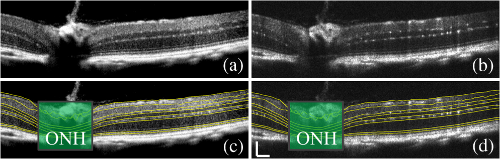$200 μ m$ .

3.1.

Segmentation of the Retinal Layers in the Mouse Eye

To observe the microvasculature network, each of the retinal layers, NFL, IPL/INL, OPL, ELM, and IS/OS of the OCT structural image [Fig. 8(a)] was successfully segmented by use of the algorithm described above. After segmentation, a number of useful presentations of the dataset can be easily generated, including a projection view or thickness map for each layer. Figures 8(b) to 8(e), respectively, show the projection views on the $X Y$ plane (i.e., en face view) for the NFL, IPL/INL, OPL, and IS/OS layers, where the anatomical features in each layer can be readily appreciated. For example, the sparse nerve fiber bundles (typical in a mouse retina) can be visualized in the NFL [Fig. 8(b)]. Although the system used to capture the mouse retinal images was of low spatial resolution ( $\sim 7 μ m$ ), the appearance of the en face view of the IS/OS layer [Fig. 8(e)] most likely corresponds to the distribution of murine photoreceptors. The user-guided segmentation is robust and works especially well at locations where the boundaries of the retinal layers are of low contrast. In particular, the interface between GCL and IPL is of low contrast, and most prior segmentation methods have had difficulty obtaining satisfactory segmentation of the IPL layer. However, using the layer-DLM to trace the IPL, the IPL was successfully obtained in our study. Finally, we can also observe the microvasculature network from within the different layers of the retina [e.g., Figs. 8(b), 8(c), and 8(d)]. Because OMAG provides the microstructure and microcirculation images in parallel, we can apply the segmentation results obtained from the microstructure images (Fig. 8) to the corresponding blood flow images in order to achieve depth-resolved vascular mapping. The results are shown in Fig. 9, where the vascular network of each layer, NFL, IPL/INL, and OPL, is clearly delineated.

Fig. 8

Segmentation results of the retinal layers in the mouse eye. (a) Segmented layers of NFL, inner plexiform layer (IPL)/INL, outer plexiform layer (OPL), external limiting membrane, and inner/outer segments (IS/OS) are presented in color and other layers are presented in grayscale. (b) to (e) Projection views of NFL, IPL/INL, and OPL layers in an OMAG image. Scale bar: $200 μ m$ .

Fig. 9

Segmentation enables visualization of vascular networks within three distinct layers: (a) NFL+ganglion cell layer (GCL), (b) IPL, and (c) OPL.

From the segmentation results shown in Fig. 8, it is a straightforward process to provide quantitative thickness maps of NFL and NFL+GCL+IPL. Figure 10 provides these quantitative results. Note that in the quantification of mouse retina, the values have accounted for the scaling factor that was used to generate images with an appropriate size to facilitate the segmentation procedures as described above. In the mouse NFL, the vessels and nerve fiber bundles coexist. Using the blood vessel information provided by the OMAG blood flow images, we are able to separate the vessels [red color in Fig. 10(a)] from nerve fiber bundles [blue color in Fig. 10(a)]. To radially quantify the retinal layer thickness variation from the ONH, the mean thickness of each region demarcated by concentric circles (100 pixels or $\sim 390 μ m$ in width) from the center of ONH to the peripheral retina was computed and provided in Figs. 10(b) and 10(c) for the NFL and NFL+GCL+IPL layers, respectively. The thicknesses of the NFL and NFL+GCL+IPL layers gradually become reduced proceeding from the ONH to the periphery, which is consistent with previously published observations.²²^,²³

Fig. 10

Retinal layer thickness map of the mouse eye. (a) Segmentation results of NFL and NFL+GCL+IPL. (b) Thickness of NFL. (c) Thickness of NFL+GCL+IPL. Unit in image is $μ m$ . Scale bar: $200 μ m$ .

3.2.

Segmentation of the Retinal Layers in 3-D OCT Image from Normal Human Subject

The OMAG images of a healthy human retina were successfully segmented into the NFL, GCL+IPL, IPL/INL, OPL, and IS/OS layers [see Fig. 11(a)]. The corresponding projection maps of the NFL, GCL+IPL, IPL/INL, OPL, and IS/OS layers are presented in Figs. 11(b) to 11(f), respectively. The GCL layer was obtained from the region between the bottom boundary of the NFL and the top boundary of the IPL. The NFL, GCL, and IPL layers merge into one common layer near the fovea [see insert of Fig. 11(a)]. Similar to the information obtained from the mouse retina, distinct physiological features within the human retina can be readily appreciated. The orientation and alignment of the nerve fiber bundles within the NFL [Fig. 11(b)] can be visualized, as well as the photoreceptor distribution within the IS/OS layer [Fig. 11(f)], which is of high density within the fovea region and gradually reduces radially outward. Such information can be critically important in understanding the diagnosis, treatment, and prognosis of patients affected by retinal diseases, such as age-related macular degeneration (AMD) and diabetic retinopathy. With the OMAG blood flow dataset, we also successfully segmented the microvascular networks located in three different layers within the retina, the GCL+IPL [Fig. 12(a)], IPL/INL [Fig. 12(b)], and OPL [Fig. 12(c)]. In contrast to the mouse retina, there are relatively large supplying arterioles and collecting venules in the human retina within the GCL+IPL layer. In particular, the blood vessel network within the OPL [Fig. 12(c)] shows simple but distinct and well-organized capillary beds in the healthy human eye. The visualization of such detailed blood vessel organization in distinct retinal layers at the true capillary level in 3-D is currently possible only with OMAG imaging technology and is also relevant to understanding the pathophysiology, treatment, and prognosis of patients affected by glaucoma, AMD, and diabetic retinopathy.⁴⁶^,⁴⁷

Fig. 11

Segmentation of the healthy human retina. From the segmented results about retinal layer boundaries (a), the en face projection views of (b) NFL, (c) GCL+IPL, (d) IPL/INL, (e) OPL, and (f) IS/OS were obtained. Scale bar: $200 μ m$ .

Fig. 12

Depth-resolved microvascular networks within (a) GCL, (b) IPL, and (c) OPL layers of the human retina. Scale bar: $200 μ m$ .

The thickness maps of each of the human retinal layers are readily available from the 3-D dataset after segmentation using the user-guided algorithm. Figure 13 illustrates the thickness maps from the NFL, NFL+GCL+IPL, and the whole retina (from NFL to IS/OS). At the location of the fovea, the NFL cannot be identified as one single layer in the OCT image and it merges with the GCL and IPL. Thus, the NFL near the fovea is artificially thicker than the actual thickness of the NFL [see gray part in Fig. 13(a)]. The mean thickness in each of the circumferential regions is 100 pixels ( $\sim 333 μ m$ ) in width from the center of the fovea to the periphery as shown. The retinal thickness decreases radially from the fovea to the periphery for the computed layers.

Fig. 13

Retinal layer thickness map of the healthy human eye. (a) Thickness of NFL. The thickness with gray background is not the thickness of the NFL but is the thickness of the fovea region. (b) Thickness of NFL+GCL+IPL. Unit in image is $μ m$ .

3.3.

Segmentation of the Retinal Layers in 3-D OCT Images from Pathological Eye

As mentioned above, segmenting the retinal layers in patient eyes in clinical practice still heavily depends on manual segmentation largely due to the challenge faced by currently available automatic segmentation algorithms. Our user-guided segmentation method was tested on the images acquired from various patient eyes scanned by both the OCT/OMAG system and a commercial OCT system. Here we show an example of the segmentation result for the images acquired from an eye with exudative AMD that presents subretinal fluid, retinal pigment epithelium (RPE) detachment, and subretinal lipid deposits, resulting in progressive blurring of the central visual acuity. From the 3-D OCT image, the ELM and RPE were obtained using layer-DLM tracing; then the IS/OS layer was obtained using the bottom boundary of the ELM and the top boundary of the RPE. The segmented results are shown in Fig. 14, where we successfully segmented the NFL, GCL+IPL, IPL/INL, OPL, IS/OS, and RPE layers [Figs. 14(b) to 14(g)]. After quantifying the segmented IS/OS layer, it is easy to calculate that the size of the exudate is $1.65 \times 10^{6} μ m^{2}$ and its volume is $3.9 \times 10^{7} μ m^{3}$ . It is interesting that there are some bright spots seen in the fluid space [arrow in Fig. 14(f)], which most likely correspond to the lipid deposits. In addition, the bright spots evident in the en face RPE image [pointed in Fig. 14(g)] may demonstrate the ability of OCT to visualize the development of subretinal hemorrhages from choroidal neovascularization that is often the sign seen in the clinic. Figure 14(h) gives the 3-D rendering of the segmented results, providing information about the precise size, volume, orientation, and location of the exudate in this patient.

Fig. 14

Segmentation of 3-D image from an exudative age-related macular degeneration eye. (a) A representative segmentation results in one cross-section image, where the image in the bottom shows a zoomed view of the region square marked in the top image. From the segmented retinal layer boundaries, the en face projection images of (b) NFL, (c) GCL+IPL, (d) IPL/INL, (e) OPL, (f) IS/OS, and (f) retinal pigment epithelium were obtained. (h) The 3-D rendering of the segmented results. Scale bar: $200 μ m$ .

The thicknesses of the NFL and NFL+GCL+IPL in the AMD patient eye were also computed (see Fig. 15). Compared to the thickness of the retinal layer in the healthy human eye (Fig. 13), the thicknesses of the NFL and NFL+GCL+IPL in the pathological eye become thinner on the average. All the information provided by the successful segmentation of the proposed user-guided algorithm would be very useful in the analyses of the microstructural changes that would aid clinical diagnosis, treatment, and management of disease.

Fig. 15

Retinal layer thickness map of the patient eye. (a) Thickness of the NFL. Note that the thickness with gray background is the thickness of the fovea region, not the thickness of the NFL. (b) Thickness of the NFL+GCL+IPL. Unit in image is $μ m$ .

3.4.

Discussion

To evaluate the accuracy of the proposed segmentation method, we compared the results of manual segmentation with those from our user-guided segmentation protocol. Five graders, who were experts in OCT imaging in ophthalmology, conducted manual segmentation on 100 images of 2-D B-scans, randomly selected from six 3-D scans of mouse and four 3-D scans of human eyes. The mean position of the boundary lines of the five manual segmentations was computed and considered as the correct segmentation (gold standard). The mean of the absolute errors of the user-guided segmentation and its standard deviation were computed for the mouse and human retinas, in pixels and in microns, using the software program SPSS20 (Table 1). In all layers, the absolute error is smaller than 1 pixel ( $\sim 4 μ m$ ), except for the NFL in the murine retina and the IPL/INL layer in the human retina, where it is slightly more than 1 pixel. This error would be acceptable for an OCT imaging system that typically has a spatial resolution of $< 10 microns$ , demonstrating the robustness of the proposed user-guided segmentation. Finally, the difference between the user-guided segmentation value and the mean of the five manual segmentation values for each of the 60 mouse retina and 40 human retina images is noted to be within 2 standard deviations (95% confidence interval) for each retinal layer. In the vast majority of images, the differences between the user-guided versus manual segmentation results were $< 2 pixels$ . Together, these results confirm the accuracy of the user-guided segmentation protocol in comparison to consistent manual segmentation values in both mouse and human OCT retina images.

Table 1

Absolute error of user-guided segmentation.

	Mouse retina OMAG images ( $n = 60$ )		Human retina OMAG images ( $n = 40$ )
Layers	$Mean \pm Std$ (pixels)	$Mean \pm Std$ (microns)	$Mean \pm Std$ (pixels)	$Mean \pm Std$ (microns)
Nerve fiber layer	$1.00 \pm 1.01$	$4.00 \pm 4.04$	$0.85 \pm 0.48$	$3.40 \pm 1.92$
Inner plexiform layer/INL	$0.96 \pm 0.57$	$3.84 \pm 2.28$	$1.05 \pm 0.61$	$4.20 \pm 2.44$
Outer plexiform layer	$0.86 \pm 0.50$	$3.44 \pm 2.00$	$0.90 \pm 0.53$	$3.60 \pm 2.12$
External limiting membrane	$0.35 \pm 0.27$	$1.40 \pm 1.08$	$0.37 \pm 0.29$	$1.48 \pm 1.16$
Inner/outer segments	$0.44 \pm 0.30$	$1.76 \pm 1.20$	$0.46 \pm 0.32$	$1.84 \pm 1.28$

OMAG, optical micro-angiography.

The current implementation of the algorithm was carried out using a computer with a 3 GHz CPU and 4G memory. The program was coded with C++ based on the image processing library OpenCV. A drawback of the current method is that the processing time is relatively long. This is because the user is required to navigate the B-scan image through a 3-D dataset onto which the user would be able to instruct the program to correct the areas of likely erroneous segmentation. We tested the user-guided segmentation program using various 3-D eye images with 400 B-scans in each 3-D dataset captured by both the commercial OCT and OMAG/OCT. The segmentation time for an entire 3-D dataset ranged from $\sim 3 \min$ (normal eyes) to $\sim 30 \min$ (eyes with severe pathological signs) depending on the quality of the B-scan images. For high-quality images from normal subjects, the layer tracking is almost automatic. However, when the quality of the images from patients is low and the boundary between the retinal layers is difficult to identify, the user needs to intervene to place user-defined lines and interactively correct the erroneous segmentation, which increases the time used. Compared to pure manual segmentation (typically 3 to 4 h), the user-guided segmentation is, however, much more efficient.

By providing a number of user-defined lines around layers or features within the 3-D OCT images, the user-guided method shows reliable and satisfactory segmentation of the retinal layers in images with complex shapes, holes, and low contrast layer boundaries. Furthermore, the user can also correct an incorrect segmentation by modifying the adaptive line using the user-guided segmentation method. As a drawback of assigning the user-defined lines, an artificial layer structure may be generated at the region where there is no layer, e.g., at the ONH and fovea regions. This artifact, however, can be easily corrected by interactively assigning the region where there is no known retinal layer on a 2-D en face image (see the gray ellipse region on thickness images in Figs. 10, 13, and 15).

In the future, two approaches will be considered to improve the performance of the current user-guided segmentation system. One approach is to develop an interpolating algorithm between user-defined lines so that it is possible to quickly construct the 3-D surface, saving user operation time. Another approach is to improve the automated layer tissue and edge detectors. Current robust DLMs can be migrated into an advanced computing platform, e.g., GPU, for further improvement of the overall performance of the proposed algorithm. When developed and clinically validated, we hope that the proposed semiautomatic strategy will have an impact on the current clinical practice of functional OCT imaging of the retina.

4. Conclusion

We have proposed a user-guided segmentation method in which the user can provide a number of defined lines around the layers and features within 3-D OCT images to guide the program to perform robust detection of the boundaries and layers of retinal layers. We have demonstrated, through implementation of the algorithms on retinal OCT images of both mouse and human eyes, that the system is reliable and efficient. The proposed approach will be useful with the current usage of OCT imaging systems because it can serve in filling the gap between current automated segmentation techniques and obtaining accurate measurements for use in clinical practice.

Acknowledgments

The authors would like to acknowledge Leona Ding for statistical guidance. This work was supported in part by research grant from National Eye Institute (R01EY024158). Dr. Wang is a recipient of an innovative award from Research to Prevent Blindness.

References

1.

W. Drexleret al., “Ultrahigh-resolution ophthalmic optical coherence tomography,” Nat. Med., 7 (4), 502 –507 (2001). http://dx.doi.org/10.1038/86589 1078-8956 Google Scholar

2.

P. H. TomolinsR. K. Wang, “Theory, developments and applications of optical coherence tomography,” J. Phys. D: Appl. Phys., 38 (15), 2519 –2535 (2005). http://dx.doi.org/10.1088/0022-3727/38/15/002 JPAPBE 0022-3727 Google Scholar

3.

G. J. JaffeJ. Caprioli, “Optical coherence tomography to detect and manage retinal disease and glaucoma,” Am. J. Ophthalmol., 137 (1), 156 –169 (2004). http://dx.doi.org/10.1016/S0002-9394(03)00792-X AJOPAA 0002-9394 Google Scholar

4.

K. H. Kimet al., “Monitoring mouse retinal degeneration with high-resolution spectral-domain optical coherence tomography,” J. Vis., 8 (1), 1 –11 (2008). http://dx.doi.org/10.1167/8.1.17 1534-7362 Google Scholar

5.

G. Huberet al., “Spectral domain optical coherence tomography in mouse models of retinal degeneration,” Invest. Ophthalmol. Vis. Sci., 50 (12), 5888 –5895 (2009). http://dx.doi.org/10.1167/iovs.09-3724 IOVSDA 0146-0404 Google Scholar

6.

Z. Zhiet al., “Noninvasive imaging of retinal morphology and microvasculature in obese mice using optical coherence tomography and optical microangiography,” Invest. Ophthalmol. Vis. Sci., 55 (2), 1024 –1030 (2014). http://dx.doi.org/10.1167/iovs.13-12864 IOVSDA 0146-0404 Google Scholar

7.

V. J. Srinivasanet al., “Noninvasive volumetric imaging and morphometry of the rodent retina with high-speed, ultrahigh-resolution optical coherence tomography,” Invest. Ophthalmol. Vis. Sci., 47 (12), 5522 –5528 (2006). http://dx.doi.org/10.1167/iovs.06-0195 IOVSDA 0146-0404 Google Scholar

8.

V. Guedeset al., “Optical coherence tomography measurement of macular and nerve fiber layer thickness in normal and glaucomatous human eyes,” Ophthalmology, 110 (1), 177 –189 (2003). http://dx.doi.org/10.1016/S0161-6420(02)01564-6 OPANEW 0743-751X Google Scholar

9.

M. R. Heeet al., “Optical coherence tomography of age-related macular degeneration and choroidal neovascularization,” Ophthalmology, 103 (8), 1260 –1270 (1996). http://dx.doi.org/10.1016/S0161-6420(96)30512-5 OPANEW 0743-751X Google Scholar

10.

A. Martidiset al., “Intravitreal triamcinolone for refractory diabetic macular edema,” Ophthalmology, 109 (5), 920 –927 (2002). http://dx.doi.org/10.1016/S0161-6420(02)00975-2 OPANEW 0743-751X Google Scholar

11.

D. C. DeBuc, “A review of algorithms for segmentation of retinal image data using optical coherence tomography,” Image Segmentation, 14 –54 InTech(2011). Google Scholar

12.

R. KafiehH. RabbaniS. Kermani, “A review of algorithms for segmentation of optical coherence tomography from retina,” J. Med. Signals Sens., 3 (1), 45 –60 (2013). Google Scholar

13.

D. C. FernandezH. M. SalinasC. A. Puliafito, “Automated detection of retinal layer structures on optical coherence tomography images,” Opt. Express, 13 (25), 10200 –10216 (2005). http://dx.doi.org/10.1364/OPEX.13.010200 OPEXFF 1094-4087 Google Scholar

14.

D. KoozekananiK. BoyerC. Roberts, “Retinal thickness measurements from optical coherence tomography using a Markov boundary model,” IEEE Trans. Med. Imaging, 20 (9), 900 –916 (2001). http://dx.doi.org/10.1109/42.952728 ITMID4 0278-0062 Google Scholar

15.

M. A. Mayeret al., “Retinal nerve fiber layer segmentation on FD-OCT scans of normal subjects and glaucoma patients,” Biomed. Opt. Express, 1 (5), 1358 –1383 (2010). http://dx.doi.org/10.1364/BOE.1.001358 BOEICL 2156-7085 Google Scholar

16.

Q. Yanget al., “Automated layer segmentation of macular OCT images using dual-scale gradient information,” Opt. Express, 18 (20), 21293 –21307 (2010). http://dx.doi.org/10.1364/OE.18.021293 OPEXFF 1094-4087 Google Scholar

17.

V. Kajicet al., “Robust segmentation of intraretinal layers in the normal human fovea using a novel statistical model based on texture and shape analysis,” Opt. Express, 18 (14), 14730 –14744 (2010). http://dx.doi.org/10.1364/OE.18.014730 OPEXFF 1094-4087 Google Scholar

18.

K. A. Vermeeret al., “Automated segmentation by pixel classification of retinal layers in ophthalmic OCT images,” Biomed. Opt. Express, 2 (6), 1743 –1756 (2011). http://dx.doi.org/10.1364/BOE.2.001743 BOEICL 2156-7085 Google Scholar

19.

M. K. Garvinet al., “Intraretinal layer segmentation of macular optical coherence tomography images using optimal 3-D graph search,” IEEE Trans. Med. Imaging, 27 (10), 1495 –1505 (2008). http://dx.doi.org/10.1109/TMI.2008.923966 ITMID4 0278-0062 Google Scholar

20.

H. Zhuet al., “FloatingCanvas: quantification of 3D retinal structures from spectral-domain optical coherence tomography,” Opt. Express, 18 (24), 24595 –24610 (2010). http://dx.doi.org/10.1364/OE.18.024595 OPEXFF 1094-4087 Google Scholar

21.

X. Zhanget al., “Automated segmentation of intramacular layers in Fourier domain optical coherence tomography structural images from normal subjects,” J. Biomed. Opt., 17 (4), 046011 (2012). http://dx.doi.org/10.1117/1.JBO.17.4.046011 JBOPFO 1083-3668 Google Scholar

22.

M. K. Garvinet al., “Automated 3-D intraretinal layer segmentation of macular spectral-domain optical coherence tomography images,” IEEE Trans. Med. Imaging, 28 (9), 1436 –1447 (2009). http://dx.doi.org/10.1109/TMI.2009.2016958 ITMID4 0278-0062 Google Scholar

23.

A. Mishraet al., “Intra-retinal layer segmentation in optical coherence tomography images,” Opt. Express, 17 (26), 23719 –23728 (2009). http://dx.doi.org/10.1364/OE.17.023719 OPEXFF 1094-4087 Google Scholar

24.

S. J. Chiuet al., “Automatic segmentation of seven retinal layers in SDOCT images congruent with expert manual segmentation,” Opt. Express, 18 (18), 19413 –19428 (2010). http://dx.doi.org/10.1364/OE.18.019413 OPEXFF 1094-4087 Google Scholar

25.

P. P. Srinivasanet al., “Automatic segmentation of up to ten layer boundaries in SD-OCT images of the mouse retina with and without missing layers due to pathology,” Biomed. Opt. Express, 5 (2), 348 –365 (2014). http://dx.doi.org/10.1364/BOE.5.000348 BOEICL 2156-7085 Google Scholar

26.

S. J. Chiuet al., “Validated automatic segmentation of AMD pathology including drusen and geographic atrophy in SD-OCT images,” Invest. Ophthalmol. Vis. Sci., 53 (1), 53 –61 (2012). http://dx.doi.org/10.1167/iovs.11-7640 IOVSDA 0146-0404 Google Scholar

27.

R. Kafiehet al., “Intra-retinal layer segmentation of 3D optical coherence tomography using coarse grained diffusion map,” Med. Image Anal., 17 (8), 907 –928 (2013). http://dx.doi.org/10.1016/j.media.2013.05.006 MIAECY 1361-8415 Google Scholar

28.

P. A. Yushkevichet al., “User-guided 3D active contour segmentation of anatomical structures: significantly improved efficiency and reliability,” Neuroimage, 31 (3), 1116 –1128 (2006). http://dx.doi.org/10.1016/j.neuroimage.2006.01.015 NEIMEF 1053-8119 Google Scholar

29.

P. W. de Bruinet al., “Interactive 3D segmentation using connected orthogonal contours,” Comput. Biol. Med., 35 (4), 329 –346 (2005). http://dx.doi.org/10.1016/j.compbiomed.2004.02.006 CBMDAW 0010-4825 Google Scholar

30.

L. AnR. K. Wang, “In vivo volumetric imaging of vascular perfusion within human retina and choroids with optical microangiography,” Opt. Express, 16 (15), 11438 –11452 (2008). http://dx.doi.org/10.1364/OE.16.011438 OPEXFF 1094-4087 Google Scholar

31.

L. Anet al., “High resolution wide-field imaging of retinal and choroidal blood perfusion with optical microangiography,” J. Biomed. Opt., 15 (2), 026011 (2010). http://dx.doi.org/10.1117/1.3369811 JBOPFO 1083-3668 Google Scholar

32.

L. Anet al., “High speed spectral domain optical coherence tomography for retinal imaging at 500,000 A-lines per second,” Biomed. Opt. Express, 2 (10), 2770 –2783 (2011). http://dx.doi.org/10.1364/BOE.2.002770 BOEICL 2156-7085 Google Scholar

33.

L. AnT. T. ShenR. K. Wang, “Using ultrahigh sensitive optical microangiography to achieve comprehensive depth resolved microvasculature mapping for human retina,” J. Biomed. Opt., 16 (10), 106013 (2011). http://dx.doi.org/10.1117/1.3642638 JBOPFO 1083-3668 Google Scholar

34.

R. K. WangL. An, “Multifunctional imaging of human retina and choroid with 1050 nm spectral domain optical coherence tomography at 92 kHz line scan rate,” J. Biomed. Opt., 16 (5), 050503 (2011). http://dx.doi.org/10.1117/1.3582159 JBOPFO 1083-3668 Google Scholar

35.

Z. Zhiet al., “Optical microangiography of retina and choroid and measurement of total retinal blood flow in mice,” Biomed. Opt. Express, 3 (11), 2976 –2986 (2012). http://dx.doi.org/10.1364/BOE.3.002976 BOEICL 2156-7085 Google Scholar

36.

X. Yinet al., “Extracting cardiac shapes and motion of the chick embryo heart outflow tract from 4D optical coherence tomography images,” J. Biomed. Opt., 17 (9), 096005 (2012). http://dx.doi.org/10.1117/1.JBO.17.9.096005 JBOPFO 1083-3668 Google Scholar

37.

P. Liet al., “Measurement of strain and strain rate in embryonic chick heart in vivo using spectral domain optical coherence tomography,” IEEE Trans. Biomed. Eng., 58 (8), 2333 –2338 (2011). http://dx.doi.org/10.1109/TBME.2011.2153851 IEBEAX 0018-9294 Google Scholar

38.

A. Liuet al., “Biomechanics of the chick embryonic heart outflow tract at HH18 using 4D optical coherence tomography imaging and computational modeling,” PloS One, 7 (7), e40869 (2012). http://dx.doi.org/10.1371/journal.pone.0040869 1932-6203 Google Scholar

39.

J. A. Tyrrellet al., “Robust 3-D modeling of vasculature imagery using superellipsoids,” IEEE Trans. Med. Imaging, 26 (2), 223 –237 (2007). http://dx.doi.org/10.1109/TMI.2006.889722 ITMID4 0278-0062 Google Scholar

40.

H. V. Poor, An Introduction to Signal Detection and Estimation, 2nd ed.Springer, New York, NY (1994). Google Scholar

41.

R. K. Wanget al., “Three dimensional optical angiography,” Opt. Express, 15 (7), 4083 –4097 (2007). http://dx.doi.org/10.1364/OE.15.004083 OPEXFF 1094-4087 Google Scholar

42.

R. K. WangS. Hurst, “Mapping of cerebrovascular blood perfusion in mice with skin and cranium intact by optical micro-angiography at 1300 nm wavelength,” Opt. Express, 15 (18), 11402 –11412 (2007). http://dx.doi.org/10.1364/OE.15.011402 OPEXFF 1094-4087 Google Scholar

43.

R. K. Wang, “Optical microangiography: a label free 3D imaging technology to visualize and quantify blood circulations within tissue beds in vivo,” IEEE J. Sel. Topics Quantum Electron., 16 (3), 545 –554 (2010). http://dx.doi.org/10.1109/JSTQE.2009.2033609 IJSQEN 1077-260X Google Scholar

44.

R. K. Wanget al., “Depth-resolved imaging of capillary networks in retina and choroid using ultrahigh sensitive optical microangiography,” Opt. Lett., 35 (9), 1467 –1469 (2010). http://dx.doi.org/10.1364/OL.35.001467 OPLEDP 0146-9592 Google Scholar

45.

L. AnJ. QinR. K. Wang, “Ultrahigh sensitive optical microangiography for in vivo imaging of microcirculations within human skin tissue beds,” Opt. Express, 18 (8), 8220 –8228 (2010). http://dx.doi.org/10.1364/OE.18.008220 OPEXFF 1094-4087 Google Scholar

46.

E. Ondaet al., “Microvasculature of the human optic nerve,” Am. J. Ophthalmol., 120 (1), 92 –102 (1995). AJOPAA 0002-9394 Google Scholar

47.

D. Y. ZhaoG. A. Cioffi, “Anterior optic nerve microvascular changes in human glaucomatous optic neuropathy,” Eye, 14 445 –449 (2000). http://dx.doi.org/10.1038/eye.2000.129 12ZYAS 0950-222X Google Scholar

Biographies of the authors are not available.

CC BY: © The Authors. Published by SPIE under a Creative Commons Attribution 4.0 Unported License. Distribution or reproduction of this work in whole or in part requires full attribution of the original publication, including its DOI.

Citation Download Citation

Xin Yin, Jennifer R. Chao, and Ruikang K. Wang "User-guided segmentation for volumetric retinal optical coherence tomography images," Journal of Biomedical Optics 19(8), 086020 (22 August 2014). https://doi.org/10.1117/1.JBO.19.8.086020

Published: 22 August 2014

Access the abstract

JOURNAL ARTICLE
10 PAGES

DOWNLOAD PAPER SAVE TO MY LIBRARY

GET CITATION

CITATIONS

Cited by 117 scholarly publications and 4 patents.

Explore citations on Lens.org

KEYWORDS

Image segmentation

Optical coherence tomography

3D image processing

Retina

Eye

Detection and tracking algorithms

Algorithm development

1.

Introduction