|
|
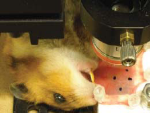
1.IntroductionOptical coherence tomography (OCT) is a noninvasive imaging modality based on the principle of low-coherence interferometry. A typical OCT system consists of an arrangement similar to a Michelson’s interferometer, where light from a low-coherence source is split into two arms: the reference arm and the sample arm. In a fiber-based implementation of OCT, the light in the reference arm is directed back after reflection from a mirror to a fiber coupler, where it gets combined with the backscattered light from the sample in the sample arm, to generate an interference fringe pattern, which can be processed to obtain the depth reflectivity profile of the sample. Data from an OCT system are typically presented in the form of two-dimensional (2-D) images called B-scans, in which the lateral and axial dimensions correspond, respectively, to the sample’s spatial dimension perpendicular (along the surface) and parallel (along depth) to the light beam. The depth reflectivity profiles in an OCT B-scan are called the A-lines, and several B-scans can be collated to form a three-dimensional OCT volume. The axial resolution of an OCT system is determined by the wavelength and bandwidth of the light source. The typical low-coherence light source used in an OCT system has a coherence length of to , which makes it an attractive imaging modality for high-resolution imaging of subsurface tissue structures. While the diagnostic potential of OCT in fields like ophthalmology and coronary artery diseases1,2 has been widely studied, few studies have been performed to assess the application of OCT for the diagnosis of oral malignancies; most of which are based on visual assessment of OCT B-scans by trained scorers.3–5 The approach of visually identifying changes in structural features like keratinization, epithelial thickening and proliferation, loss of basement membrane, irregular epithelial stratification, and basal hyperplasia, which are associated with the malignant transformation of the oral tissue, has a limited scope for two main reasons. First, it is extremely time consuming and practically impossible to visually evaluate the large amount of data obtained from a high-speed OCT system, and second, certain properties of tissue texture, like graininess and homogeneity, are difficult to quantify by direct visualization. Therefore, it is highly desirable to develop automated image processing methods that can characterize tissue morphology and texture in OCT images for quantitative diagnosis of oral malignancies. In the context of oral cancer, very few studies6,7 have assessed the performance of computational methods for tissue characterization. Yang et al.6 analyzed the diagnostic potential of three OCT features, namely the standard deviation of an A-line signal, the exponential decay constant of the spatial-frequency spectrum of an A-line profile, and the epithelial thickness. These features were derived from one-dimensional A-line profiles, which provide a partial characterization of an inherently 2-D OCT B-scan image. Likewise, in a recent publication, Lee et al.7 have described a metric based on the standard deviation of the intensity in an OCT B-scan, similar to the previous study, to characterize the oral tissue. To make better use of the information contained in a 2-D OCT B-scan, the standard deviation metric described was computed over a moving 2-D window to obtain a map of standard deviations for each OCT B-scan. However, the authors of this study, similar to the previous study, used a simple threshold-based approach for performing tissue classification and assessing the sensitivity and specificity of the proposed features. In this study, we present algorithms for extracting morphological features from OCT B-scans of hamster cheek pouches to quantify structural changes like the loss of layered structure and epithelial proliferation in oral tissue, which are known to be associated with the progression of oral cancer. The OCT features are subsequently used to design a statistical classification model to discriminate between samples belonging to three histological grades of carcinogenesis, namely benign, precancerous, and cancerous. To obtain an unbiased measure of classification performance, a cross-validation (CV) procedure is used, which involves multiple rounds of classifier training and testing. Finally, using a feature selection algorithm, a smaller subset of most relevant OCT features is identified and its performance is compared against the complete set of OCT features. 2.Materials and Methods2.1.Animal Model and ProtocolThe standard Syrian golden hamster (Mesocricetus auratus) cheek pouch model of epithelial cancer was used in this study. The animal protocol consisted of scheduled application of a suspension of 2.0% benzo[a]pyrene (Sigma Aldrich Corporation, St. Louis, Missouri) in mineral oil to the right cheek of 18 hamsters three times per week for up to 32 weeks. Eleven control animals were similarly treated with mineral oil alone. The procedure was approved by the Institution for Animal Care and Use Committee at Texas A&M University. Before imaging, the hamsters were anaesthetized by an intraperitoneal injection of a mixture of ketamine and xylazine. The cheek pouches of the anaesthetized animals were inverted and positioned under the microscope objective of the imaging system. OCT volumes were acquired from different locations on the check pouch, which were marked with tissue ink to allow the correlation between the imaging and biopsy sites, as shown in Fig. 1. After imaging, the animal was euthanized by barbiturate overdose. 2.2.Imaging SystemThe Fourier-domain OCT system used in this study was based around a 830-nm (40-nm full width at half maximum) superluminescent light-emitting diode (SLED) (EXS8410-2413, Exalos, Langhome, Pennsylvania) as the light source, providing an axial resolution of (in air). Light from the SLED was directed to a optical fiber coupler through a single-mode fiber, where it was split into reference and sample arms. The reflected beam from the reference mirror and the backscattered light from the sample were recombined at the fiber coupler, and the spectral interferogram was obtained using a custom-designed grating-based high-speed spectrometer (, Wasatch Photonics, Logan, Utah; bandwidth: 102 nm) and a CCD line-scan camera (Aviiva, SM2CL1014, EV2 Technologies, Essex, England; line rate up to 53 kHz). The detected signal was acquired and digitized using a high-speed imaging acquisition board (PCIe-1427, National Instruments, Austin, Texas). The OCT system had a sensitivity of 98 dB (defined by the system SNR of a perfect reflector) and a 3-dB single-sided fall-off of . Beam scanning over a field of view of [corresponding to () pixels] was achieved using a set of galvo mirrors (6230H, Cambridge Technology, Lexington, Massachusetts). Standard Fourier-domain OCT signal processing, involving conversion from to -space, resampling, and Fourier transform, was performed in MATLAB (The Mathworks, Inc., Natick, Massachusetts). 2.3.Histological EvaluationBiopsy samples from the imaged areas were processed following the standard procedures for histopathology analysis (H&E staining). On average, 10 sections per tissue sample were obtained and each section was assessed by a board-certified pathologist to be one of the following five grades: (1) normal (G0), (2) hyperplasia and hyperkeratosis (G1), (3) hyperplasia with dysplasia (G2), (4) carcinoma in situ (G3), and (5) squamous cell carcinoma (G4). For classification analysis, the following criteria (listed in Table 1) were used to assign class labels to each tissue sample: (1) class 1 (benign; 22 samples): samples from the control group (15 samples) and samples for which all histology sections were graded as G1 (7 samples); (2) class 2 (precancerous; 12 samples): samples for which at least 50% sections were graded as G2 or G3 and none of the sections were graded as G4; and (3) class 3 (cancerous; 14 samples): samples for which all sections were graded as G4. Samples that could not be assigned to any of the above-mentioned classes were excluded from the analysis. Table 1Summary of histopathological assessment and class assignment for different samples. 2.4.OCT FeaturesProgression of oral cancer is associated with several structural modifications of the oral tissue such as loss of the layered structure, irregular epithelial stratification, and epithelial infiltration by immature cells. As can be seen in Fig. 2(a), different layers of normal oral tissue can be easily identified in an OCT B-scan. Stratum corneum, the topmost kertainized layer of the oral tissue, can be seen as a bright layer at the air–tissue interface. Just below this layer, a dark band corresponding to the stratified squamous epithelium can be seen. Finally, the epithelium layer is followed by the lamina propria, the top portion of which appears as a region of bright intensity. In contrast, as shown in Fig. 2(b), B-scan of a malignant oral tissue shows an absence of the layered structure. The B-scan of a malignant tissue can be seen to have the brightest intensity at the surface that gradually fades off with depth. Likewise, the presence of epithelial cell infiltration in malignant oral tissue manifests as an interspersed speckled region in an OCT B-scan as shown in the inset in Fig. 2(b), whereas the epithelial region in a B-scan of a normal tissue appears as a low-intensity region flanked on either side by regions of high intensity [inset in Fig. 2(a)]. To characterize these differences in tissue morphology between normal and malignant tissues, we evaluated two sets of OCT features, which shall be referred to as the A-line derived features and B-scan derived features. Fig. 2Textural differences between B-scans of a normal tissue and a malignant tissue [(a) and (b), respectively]. Different layers of the oral mucosa can be clearly seen in the normal tissue as opposed to the malignant tissue, where the layered structure of the tissue is absent. Magnified views of portions of the epithelial regions (insets) show the continuous dark and bright bands in the case of a normal tissue versus an interspersed speckled region for the malignant tissue. 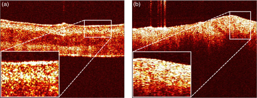 2.4.1.A-line derived featuresAs shown in Fig. 3 (top left), an A-line of a normal oral tissue shows multiple prominent peaks corresponding to the different layers of the oral mucosa, whereas for a nonlayered tissue, there is only one prominent peak corresponding to the tissue surface (top right). To quantify these characteristics of A-lines, we defined two types of A-line features, which shall be referred to as the “peaks and valleys” and “crossings” features. Fig. 3Schematic illustrating the process of obtaining peaks and valleys and crossings features from representative A-lines from a normal oral tissue (left column) and a squamous cell carcinoma tumor tissue (right column). The top row shows the raw A-lines that were filtered to remove spurious peaks and valleys. The filtered A-lines were subsequently used to compute the peaks and valleys and crossings features. The following four metrics constituted the peaks and valleys features: (1) , (2) , (3) , and (4) , where and denote the normalized intensity values of the peaks and valleys, respectively. To compute the crossings features for an A-line (bottom row), the intensity axis was partitioned into 20 equal intervals (shown as dashed lines). A crossings vector (shown as a color-coded vector; also see the legend) was defined such that the ’th element is equal to the number of times the filtered A-line intersects the ’th partition line. The mean, median, mode, and standard deviation of the elements of the crossings vector comprised the crossings features. 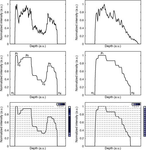 To calculate these features, the A-lines were processed using a multistep procedure outlined in Algorithm 1. Briefly, the B-scans were first filtered in the lateral direction by using a moving average kernel of size 60 to reinforce the layered structure in B-scans. Next, the A-lines were filtered, in the axial direction, by performing morphological closing (to flatten insignificant valleys), followed by opening (to eliminate narrow peaks) by flat structuring elements of size 10 and 5 pixels, respectively. The intensity values of each A-line were subsequently normalized to the range [0,1] by a simple shifting and scaling procedure. Finally, for all A-lines, any spurious peaks having a normalized magnitude of less than 0.1 were suppressed by performing the h-maxima transformation. Details about morphological opening and closing operations and h-maxima transform can be found in any standard text on morphological image processing.8 Algorithm 1Algorithm for filtering A-lines in a B-scan.
To calculate the peaks and valleys features, local maxima (peaks) and minima (valleys) of the filtered A-lines were detected and the following four peaks and valleys features were computed: (1) , (2) , (3) , and (4) , where and denote the normalized intensity values of the ’th peak and valley, respectively. This is illustrated in Fig. 3 (middle row). To calculate the crossings features, a crossings vector of size was defined for each A-line, such that the ’th element of the crossings vector is equal to the number of times the filtered A-line would intersect an imaginary line drawn parallel to the -axis (depth) and having a coordinate (normalized intensity value) of [shown as dashed lines in Fig. 3 (bottom row)]. Intuitively, if an A-line has just one prominent peak, then all the elements of the crossings vector would be two, whereas for an A-line that has multiple prominent peaks, several elements of the crossings vector would be greater than two, as shown in Fig. 3. Four crossings features defined as the (a) mean, (b) median, (c) mode, and (d) standard deviation of the elements of the crossings vector were computed. Overall, eight A-line derived features (four peaks and valleys and four crossings features) were obtained for each A-line, resulting in eight 2-D feature maps of size pixels for each OCT volume. 2.4.2.B-scan derived featuresSpeckle pattern in an OCT image of a tissue sample is known to contain information about the size and distribution of the subresolution tissue scatterers.9,10 Oral dysplasia is often characterized by basal cell hyperplasia and epithelial proliferation. The presence of dysplastic cells in the epithelium results in an interspersed speckle pattern in an OCT B-scan [Fig. 2(b)], which is different from the speckle pattern seen in B-scans of normal oral tissue, where different layers appear as more homogeneous bright and dark regions. To quantify this difference in speckle patterns, several B-scan derived texture features were computed. The first step in computing these features was to segment out the epithelial region in a B-scan. In the case of a layered tissue, the region between the first and the second peaks of filtered A-lines, obtained from Algorithm 1, was identified as the epithelial region. In the other extreme case, where the tissue lacks the layered structure, a simple approach based on -means clustering11 was employed to delineate the epithelial region. In this approach, outlined in Algorithm 2, a B-scan after log transformation and normalization was clustered into three groups using -means clustering algorithm. The dominant foreground region was subsequently identified as the largest connected component of the cluster containing the pixel that has the maximum intensity value. Any discontinuities in the region thus identified are eliminated by performing an image filling operation based on morphological reconstruction8 to obtain a contiguous segmented epithelial region. For B-scans that had both layered as well as nonlayered regions, the epithelial region was delineated by using the A-line based approach for the layered regions (identified as regions having A-lines with two or more peaks) or the -means based approach for the nonlayered regions (identified as regions having A-lines with only one peak). Algorithm 2Algorithm for generating a binary mask corresponding to the epithelial region in a nonlayered B-scan.
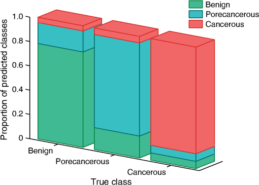
Once the epithelial region was identified, gray-level run length (GLRL)-based texture analysis was performed on the segmented region. A gray-level run is a sequence of consecutive pixels, along some direction, having the same gray-level value. The length of a gray-level run is the number of pixels in that run. To quantify the texture based on GLRL, a 2-D GLRL matrix for a given direction is computed. The element () of the GLRL matrix denotes the number of times a run of length and pixel value is found in the image. The process of obtaining a GLRL matrix for a image is illustrated in Fig. 4. To obtain texture features from a GLRL matrix, 11 different measures characterizing different textural properties, like coarseness, nonuniformity, etc.,12 were computed (Fig. 4). For an intuitive understanding, the set of 11 GLRL features can be categorized into four groups. The first group of features comprises features that characterize image texture based on the length of runs in an image. This group consists of the short run emphasis (SRE) feature, which has a higher value for images in which shorter runs as opposed to longer runs are more abundant, as in the case of a fine-grained texture. The other feature in the same group is the long run emphasis (LRE) feature, which is complimentary to the SRE feature in the sense that it has a higher value for images in which longer runs as opposed to shorter runs dominate. The second group of GLRL features consists of features that characterize image texture based on the gray-level values of runs in an image. These include the low gray-level emphasis (LGRE) and the high gray-level emphasis (HGRE) features, which increase in images that are dominated by runs of low- and high-gray values, respectively. The third group consists of four features, which are combinations of the features in the first two groups. These include short-run low gray-level emphasis (SRLGE), long-run high gray-level emphasis (LRHGE), short-run high gray-level emphasis (SRHGE), and long-run low gray-level emphasis (LRLGE) features. Finally, the fourth group of GLRL features contains features that characterize the variability of run lengths and gray levels in an image. This group contains four features, namely gray-level nonuniformity (GLNU), run length nonuniformity (RLNU), and run percentage (RP), which have self-explanatory names. The formulae to calculate these features from a run length matrix are listed in Fig. 4. Fig. 4Schematic illustrating the process of building a gray-level run length (GLRL) matrix. For a given direction (here 0 deg), the element () of the GLRL matrix denotes the number of times a run of length and pixel value is found in the image. Runs of length one, two, and three in the example image are color coded in purple, orange, and green, respectively. Formulae to compute the 11 GLRL-derived texture features are also listed. 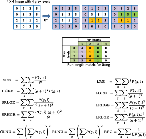 To take care of the possible slanted tissue orientation, the B-scans were aligned with respect to the air–tissue interface before computing the texture features. The GLRL features were computed for both vertical and horizontal directions and for two quantization levels, namely binary and 32 gray levels, yielding 44 B-scan–derived texture features. The GLRL texture features for each B-scan were computed over a sliding window region of size 60 A-lines within the delineated epithelial region, resulting in B-scan–derived texture feature maps of size for each OCT volume. The window size of 60 A-lines was heuristically determined to ensure that the region of interest was large enough to obtain statistically meaningful textural properties, while still being small enough to capture textural variations within a B-scan. Both the A-line– and B-scan–derived OCT feature maps were spatially averaged (window size: ) to yield a total of 52 2-D OCT feature maps of size , corresponding to a pixel resolution of . 2.5.Classifier Design and EvaluationThe objective of a classification algorithm is to assign a category or class to a new data point based on the information obtained from an available set of preclassified data points called the training set. A data point is characterized by certain attributes or features, and the problem of classifier design is that of estimating the parameters of a model describing the functional relationship between the features and class labels. The process of estimating these parameters constitutes the training phase of a classifier design. To evaluate the classification accuracy of a classifier, the trained classifier is tested to predict the class of data points in a test set which have preferably not been used for training (i.e., not included in the training set). The predicted class labels produced by the classifier are compared with the true class labels of the test data (assumed to be known) to evaluate the classification accuracy of the classifier. To evaluate the discriminatory potential of OCT features, a popular ensemble classification method called random forest was used in this study. Ensemble-based classification methods offer an attractive alternative to the traditional classification algorithms to deal with complex classification problems. An ensemble-based method, in simple terms, combines several weak classifiers to produce a strong classifier. This often results in an improved classification accuracy, which comes at the expense of a higher computational overhead. The advantages of an ensemble-based method over a single classifier have been widely studied.13 The ensemble classifier, random forest, used in this study is an ensemble of simple decision trees classifiers.14 In the context of classification algorithms, a data point characterized by features is represented as a vector in a -dimensional feature space. The process of classification for a $m$-class problem can then be thought of as partitioning the feature space into different regions. A decision tree classifier partitions the feature space into disjoint rectangular regions based on a set of recursive binary rules. This is illustrated in Fig. 5(b) for the case of a three-class problem in a 2-D feature space. The rules in the case of the example shown in Fig. 5(b) are: (1) Region 1 (green): Feature ; (2) Region 2 (red): (Feature ) and (Feature ); and (3) Region 3 (blue): (Feature ) and (Feature ). These rules are graphically represented as a tree shown in Fig. 5(a), where each split point or an internal node in a tree represents a binary question based on one of the features and the terminal nodes of the tree represent a class label. The process of training a decision tree involves determining the set of rules or the binary test conditions for each internal node of the decision tree. Classifying a test data point is straightforward once the decision tree has been built. Starting from the top-most node, the data point is propagated down the tree based on the decision taken at each internal node, until it reaches a terminal node. The class label associated with the terminal node is then assigned to the test data point. Fig. 5Classification by random forest. (a) Graphical representation of the decision process in form of a binary tree. (b) Partitioning of the feature space based on the rules of the decision tree in (a). (c) The process of training and testing of a random forest. 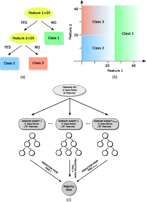 While decision trees have several advantages, like the ability to handle multiclass problems, robustness to outliers, and computational efficiency, they suffer from disadvantages such as low prediction accuracy for complex classification problems and high variance. Random forest overcomes the disadvantages of decision trees by forming an ensemble of several decision trees (denoted by here) during its training phase.15 Assuming that the training set consists of data points characterized by features, each decision tree in a random forest is trained over a set of data points obtained by sampling by replacement from the pool of training data points and features chosen randomly from the original features. In this study, we used and for training the random forest. These parameters were heuristically chosen to provide a satisfactory tradeoff between the computation time and accuracy. To classify a new data sample, the class of the data sample is first predicted by each decision tree and the final class predicted by the random forest is obtained by simply taking a majority vote of the classes predicted by individual trees. This process is illustrated in Fig. 5(c). To obtain an unbiased estimate of the classification accuracy, it is necessary to test the performance of the classifier on independent test data that has not been used for training. CV is a commonly used, powerful resampling statistical technique for estimating the generalization performance (i.e., the performance on data that has not been used for training) of an algorithm. In the context of classification, CV provides a means of obtaining an unbiased estimate for classification accuracy. In this study, a variant of the leave-one-out CV (LOO CV) method was used to estimate the classification accuracy. In the standard LOO CV procedure, all but one data points are used for training the classifier and the left-out data point is used for testing. The process of training and testing is repeated in an iterative round-robin fashion (each iteration called a fold of CV), until all the data points are used as test data points. Since the data points in our study correspond to pixels in 2-D feature maps, to avoid optimistically biased accuracy estimates resulting from spatial correlation between pixels, we performed leave-one-sample-out CV (LOSO CV), wherein CV folds were performed over the datasets and not pixels. In addition to the mean classification accuracy (obtained by averaging the accuracies obtained on individual CV folds), the classifier performance was also evaluated by computing the sensitivity and specificity for each class by pooling the results of the different CV folds. 2.6.Feature Selection for OCT FeaturesFeature selection is a process of selecting a subset of features from a large pool of features. The objective of feature selection is to remove redundant (correlated) and irrelevant features while retaining the most relevant features for building a predictive model. Getting rid of redundant and irrelevant features not only results in reduced computational cost, both in terms of training and testing the model, but also provides a better understanding of the importance of different features in the classification model. Due to the large number of correlated OCT features, we used the minimum redundancy maximum relevance (mRMR) algorithm16 to identify the most important OCT features. mRMR is a mutual information-based powerful feature selection method that aims at selecting features that are mutually different but highly relevant for classification. The choice of mRMR was motivated by its versatility in terms of its ability to (a) handle both continuous and discrete data types, (b) work with multiclass classification problems and, (c) be computationally more efficient and superior to several other feature selection methods.17 Additionally, unlike most empirical feature selection methods, mRMR is based on a sound theoretical understanding in that it can be seen as an approximation to maximize the dependency between the joint distribution of the selected features and the classification variable. The predictive power of the smaller set of OCT features obtained by mRMR algorithm was also evaluated by using training and testing procedures similar to what was used for the complete set of OCT features. 3.Results and Discussion3.1.Epithelial SegmentationResults of the segmentation algorithm to delineate the epithelial region in B-scans are presented in Fig. 6. The top row in Figs. 6(a)–6(c) shows the B-scans representative of three different cases of tissue architecture, in terms of the presence or absence of the layered structure. These cases include B-scans with (1) uniformly layered appearance [Fig. 6(a)], (2) both layered and nonlayered regions [(Fig. 6(b), layered region on the left side and nonlayered on the right side], and (3) uniformly nonlayered appearance [Fig. 6(c)]. The bottom row in Figs. 6(d)–6(f) shows the delineated top and bottom boundaries of the epithelial region, in blue and cyan, respectively, for the corresponding B-scans in the top row. It can be seen from these results that the proposed simple segmentation procedure was able to successfully identify the epithelial region in all three cases. It must be noted that to achieve the accurate segmentation of OCT image, it is desirable that the images have minimal noise. In the context of present research, this means that the OCT images corrupted by artifacts like bright stripes resulting from strong backreflections from optical components would cause the proposed segmentation algorithm to fail. Fig. 6Results of the segmentation procedure used to delineate the epithelial region in optical coherence tomography (OCT) B-scans for the case of a layered tissue [left, (a) and (d)], nonlayered tissue [right, (c) and (f)], and a tissue having both layered and nonlayered regions [center, (b) and (e)]. The epithelial region is identified as the region between the blue and cyan lines shown in the bottom row [(d)–(f)]. 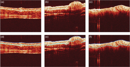 3.2.Classification Based on All OCT FeaturesResults of the random forest classification based on all OCT features are presented in Table 2 and Fig. 7. The overall classification accuracy estimated by the LOSO CV procedure was 80.6%. The sensitivity and specificity values for the three classes are presented in Table 2. The grouped bar graph shown in Fig. 7 provides further insights into the classifier performance. High values for the proportion of cancerous samples that were classified correctly are reflected in the good sensitivity for the cancerous class, whereas the relatively lower sensitivity for the benign and precancerous classes results from the confusion between the two classes. The confusion between the benign and precancerous classes could possibly be due to two reasons. First, it could be the case that the OCT features used in this study are not discriminatory enough to provide good class separation between the benign and precancerous classes. Second, the confusion between the two classes could likely be due to mislabeled data points in the training data. Recall that a sample was labeled precancerous if the histopathological evaluation of at least 50% of sections in that sample indicated the presence of some grade of dysplasia. This means that not all the pixels in a precancerous sample (although all labeled as precancerous) were truly representative of precancerous conditions. The “label noise” arising in this way could be responsible for the confusion between the benign and precancerous classes. The performance of the classifier for the binary case when the precancerous and cancerous classes are pooled together to form the malignant class was also evaluated. The overall classification accuracy in this case was 83.7%, and the sensitivity and specificity of distinguishing malignant lesions from benign lesions were found to be 90.2% and 76.3%, respectively. Table 2Diagnostic sensitivity and specificity of the optical coherence tomography (OCT) features.
3.3.Feature SelectionAs mentioned in an earlier section, mRMR feature selection method was used to obtain 52 incremental feature sets (). The sequential feature sets are ordered such that the ’th feature set, , contains the most discriminatory features. The mean classification accuracies for the sequential feature sets were subsequently computed by using a random forest–based training and testing procedure similar to what was used for the complete set of OCT features. Figure 8 shows the mean classification accuracies for the 52 sequential feature sets. The plot suggests that using more than six features does not offer a significant improvement in the mean classification accuracy; accuracy for the best six features being 0.804 compared with 0.809 (shown by black dashed line in Fig. 8) for all OCT features. Specifically, the set of six most important OCT features obtained by the mRMR algorithm included both A-line and B-scan derived features, viz.: (1) std (crossings), (2) LRLGE (90 deg, 32 bits), (3) RP (0 deg, 2 bits), (4) , (5) RP (90 deg, 32 bits), and (6) SRHGE (0 deg, 2 bits). This suggests that using both types of OCT features (A-line– and B-scan–derived features) would provide better diagnostic performance than using just one type of OCT features. From a practical standpoint, using fewer OCT features would reduce the computational cost, which includes classifier’s complexity and time required for training and testing the classification model, without any significant loss of predictive power. Fig. 8Mean classification accuracies for the sequential OCT feature sets using mRMR incremental feature selection procedure. The dashed black line denotes the mean accuracy obtained by using all 52 OCT features. 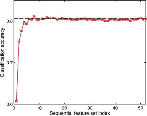 Based on previous discussions, it is worthwhile to mention that the choice of random forest as the classification method was motivated by two key considerations. First, it has been shown that the random forest–based classification is relatively more immune to the presence of noisy labels in the training dataset.18 This helps in mitigating the effect of the label noise discussed in an earlier section. Second, random forest classifiers are robust to overfitting in the case of a large number of possibly correlated features,19 which is evident from Fig. 8, where it can be seen that the LOSO CV classification accuracy does not deteriorate with increasing number of features. 4.ConclusionsNot many studies have evaluated the potential of OCT for oral cancer detection. Even fewer studies have focused on automated classification of OCT images. In this study, we presented the feasibility of using image analysis algorithms for automated characterization and classification of OCT images in a hamster cheek pouch tumor model. We recognize that the sample size used in this study was rather small, and a larger pool of samples with more diverse histological presentations is therefore warranted to fully substantiate the findings of the current study. Nevertheless, the results of the present study are encouraging and provide promise for OCT-based automated diagnosis of oral cancer. AcknowledgmentsThis work was supported by grants from the National Institutes of Health: R21-CA132433 and R01-HL11136. ReferencesM. Wojtkowskiet al.,
“Three-dimensional retinal imaging with high-speed ultrahigh-resolution optical coherence tomography,”
Ophthalmology, 112
(10), 1734
–1746
(2005). http://dx.doi.org/10.1016/j.ophtha.2005.05.023 OPANEW 0743-751X Google Scholar
I.-K. Janget al.,
“In vivo characterization of coronary atherosclerotic plaque by use of optical coherence tomography,”
Circulation, 111
(12), 1551
–1555
(2005). http://dx.doi.org/10.1161/01.CIR.0000159354.43778.69 CIRCAZ 0009-7322 Google Scholar
P. Wilder-Smithet al.,
“In vivo optical coherence tomography for the diagnosis of oral malignancy,”
Lasers Surg. Med., 35
(4), 269
–275
(2004). http://dx.doi.org/10.1002/(ISSN)1096-9101 LSMEDI 0196-8092 Google Scholar
E. S. Mathenyet al.,
“Optical coherence tomography of malignancy in hamster cheek pouches,”
J. Biomed. Opt., 9
(5), 978
–981
(2004). http://dx.doi.org/10.1117/1.1783897 JBOPFO 1083-3668 Google Scholar
W. Junget al.,
“Advances in oral cancer detection using optical coherence tomography,”
IEEE J. Sel. Top. Quantum Electron., 11
(4), 811
–817
(2005). http://dx.doi.org/10.1109/JSTQE.2005.857678 IJSQEN 1077-260X Google Scholar
C. Yanget al.,
“Effective indicators for diagnosis of oral cancer using optical coherence tomography,”
Opt. Express, 16
(20), 15847
–15862
(2008). http://dx.doi.org/10.1364/OE.16.015847 OPEXFF 1094-4087 Google Scholar
C.-K. Leeet al.,
“Diagnosis of oral precancer with optical coherence tomography,”
Biomed. Opt. Express, 3
(7), 1632
–1646
(2012). http://dx.doi.org/10.1364/BOE.3.001632 BOEICL 2156-7085 Google Scholar
P. Soille, Morphological Image Analysis: Principles and Applications, Springer-Verlag, New York
(2003). Google Scholar
K. W. Gossageet al.,
“Texture analysis of optical coherence tomography images: feasibility for tissue classification,”
J. Biomed. Opt., 8
(3), 570
–575
(2003). http://dx.doi.org/10.1117/1.1577575 JBOPFO 1083-3668 Google Scholar
A. A. Lindenmaieret al.,
“Texture analysis of optical coherence tomography speckle for characterizing biological tissues in vivo,”
Opt. Lett., 38
(8), 1280
–1282
(2013). http://dx.doi.org/10.1364/OL.38.001280 OPLEDP 0146-9592 Google Scholar
R. O. DudaP. E. HartD. G. Stork, Pattern Classification, John Wiley & Sons, New York
(2012). Google Scholar
X. Tang,
“Texture information in run-length matrices,”
IEEE Trans. Image Process., 7
(11), 1602
–1609
(1998). http://dx.doi.org/10.1109/83.725367 IIPRE4 1057-7149 Google Scholar
T. G. Dietterich,
“Ensemble methods in machine learning,”
Multiple Classifier Systems, 1
–15 Springer, Berlin, Heidelberg
(2000). Google Scholar
L. Breiman,
“Random forests,”
Mach. Learn., 45
(1), 5
–32
(2001). http://dx.doi.org/10.1023/A:1010933404324 MALEEZ 0885-6125 Google Scholar
A. Criminisi,
“Decision forests: a unified framework for classification, regression, density estimation, manifold learning and semi-supervised learning,”
Found. Trends Comput. Graph. Vision, 7
(2–3), 81
–227
(2011). http://dx.doi.org/10.1561/0600000035 1572-2740 Google Scholar
H. PengF. LongC. Ding,
“Feature selection based on mutual information criteria of max-dependency, max-relevance, and min-redundancy,”
IEEE Trans. Pattern Anal. Mach. Intell., 27
(8), 1226
–1238
(2005). http://dx.doi.org/10.1109/TPAMI.2005.159 ITPIDJ 0162-8828 Google Scholar
C. YunJ. Yang,
“Experimental comparison of feature subset selection methods,”
in Data Mining Workshops, 2007,
367
–372
(2007). Google Scholar
T. G. Dietterich,
“An experimental comparison of three methods for constructing ensembles of decision trees: bagging, boosting, and randomization,”
Mach. Learn., 40
(2), 139
–157
(2000). http://dx.doi.org/10.1023/A:1007607513941 MALEEZ 0885-6125 Google Scholar
L. Breiman,
“Random forests,”
Mach. Learn., 45
(1), 5
–32
(2001). http://dx.doi.org/10.1023/A:1010933404324 MALEEZ 0885-6125 Google Scholar
|

