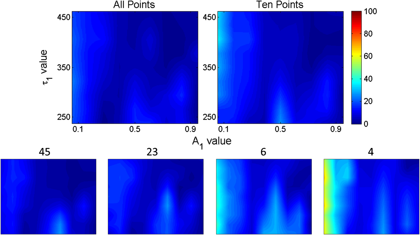
2.1.

Time-Domain Wide-Field Gated Imaging

Generally, there are two main experimental techniques employed to acquire time-domain fluorescence decay curves over the typical range of fluorophore lifetimes employed in bioimaging: time-correlated single-photon counting and time-gated detection. Time-gated techniques are preferred, especially when large field of views and fast acquisition times are desired. In this work, we used a wide-field time-gated imaging platform working in the NIR range³⁰ and employed an active illumination module.^31–33 This system has been designed to quantitatively image FRET donor fractions in vitro, ex vivo, and in vivo.^29,31,34 Briefly, the system uses a Maitai laser as a source and is coupled to a digital micromirror unit (DLP Discovery 4100 Kit and D2D module, Texas Instruments Inc., Dallas, Texas) to obtain a spatially controllable wide-field excitation [or active wide-field illumination (AWFI)]. The fluorescence signals are collected in transmittance geometry via an ultrafast-gated, intensified CCD (ICCD) camera (Picostar HR, LaVision GmbH, Goettingen, Germany) which has a 12-bit CCD and a resolution of $1376\times 1040\text{pixels}$. For all experiments herein, the gate width size was set to 300 ps, the step size between gates to 40 ps, and the camera integration time to 800 ms. These settings were kept constant for both high-throughput FRET imaging in well plates and in vivo FRET imaging described in Secs. 2.4 and 2.5, respectively.

To ensure the acquisition of optimal fluorescence decay curves in terms of signal-to-noise ratio, an active illumination strategy was employed for all experimental data employed herein. In this approach, the illumination spatial distribution is actively and iteratively optimized to yield time fluorescence decay curves with maximum photon counts near the saturation level of the ICCD (3600 counts). Overall, this method allows for enhanced accuracy in lifetime-based imaging at high acquisition speed over samples with large fluorescence intensity distributions. We previously demonstrated that AWFI is able to accurately estimate lifetimes from a multiwell plate sample with concentrations ranging over 2 orders of magnitude, resulting in estimation error in quenched donor fraction of less than 6% (compared with optimally acquired, one-by-one analysis) over 18 well samples.³³

2.2.

Biexponential and Noise Model

In the case of a population of two fluorophores with distinct lifetimes, the fluorescence decay curves can be accurately modeled using a biexponential model convolved with the IRF of the system.^35,36 In such cases, the model is expressed as

This model was used to fit experimental data as well as to generate synthetic data to investigate the impact of the number and location of time gates on the estimation of the above-mentioned fitted parameters over a large range of functional values. To derive synthetic fluorescence measurements closely mimicking experimental data, the model in Eq. (1) was augmented via additive noise. Background noise, dark noise, and photon (shot) noise are generally the primary sources of noise in time-domain measurements.³⁷ Background noise can be limited by reducing the amount of ambient light incident on the system. All background noises are unlikely to be eliminated, and it must be measured and accounted for during the fitting process (usually via subtraction). Dark noise is kept to a minimum via active cooling of the ICCD. Shot noise follows a Poisson distribution and is due to the nonconstant absorption and emission of photons in response to a mean excitation signal. Though time-gated systems are not strictly shot noise limited, McGinty et al.⁶ have shown that the shot noise-like behavior is present when using common gain voltages. In practice, when modeling these systems, Poisson noise is usually the only added noise.^38–40 Hence, an absolute Poisson noise was used as a good model for experimental noise in this study. As our experimental implementation benefits from active illumination, it yields homogeneous fluorescence time decay curves with maximum photon counts $\sim 3600$; all simulated data were normalized to this absolute count number. The Poisson noise was calculated at each gate and added to the pure fluorescence decay after convolution with the IRF to yield the synthetic data. Note that for the sake of comparison, RLD was also applied in certain cases with the formulation defined by Elangovan et al.⁴¹

2.3.

In Silico Experimental Design

When acquiring in vitro and in vivo time-gated FLIM-FRETs, a few temporal parameters need to be specified a priori. First, the gate size and the step between gates need to be defined. Conventional gated systems based on gated ICCDs allow for a gate size between 200 and 1000 ps. Two-hundred-picosecond time gates are generally unstable, whereas large time gates, even if they lead to significantly faster acquisitions,⁴² oversmooth the fluorescence decays, leading to loss of accuracy in fitting.⁴³ Herein, as described in Sec. 2.1, the gate size was set to 300 ps and the step size between gates to 40 ps in all simulations to replicate optimal experimental conditions for FRET imaging. To avoid the confusion between gate numbers and their temporal locations, only gate numbers will be referenced in the remainder of this work. Because the step size is consistent, the temporal position of any time gate can be found by multiplying the gate number by 40 ps (e.g., gate 10 is temporally located at approximately 400 ps after the peak of the decay). A total of 115 gates with equal step spacing were simulated to generate full fluorescence decay curves over a 4.6-ns temporal window. Second, when considering sparse temporal datasets, two parameters need to be defined: number of gates acquired and location of the gates. Herein, a brute-force approach based on large random trials is performed to investigate the impact of these two parameters on the estimation of FRET quantities.

First, a simulation is used to assess the information content of each individual time gate as quantified by the ${\chi }^2$ value. To limit this investigation to a workable range of parameters, synthetic decay curves were created with model parameters set to $A_1=0.3$, $A_2=0.7$, ${\tau }_1=300\mathrm{ps}$, and ${\tau }_2=1200\mathrm{ps}$. These fractional amplitudes are frequently encountered in FRET applications, whereas the two lifetimes correspond to the lifetimes of the two states of the donor in the NIR FRET pair Alexa Fluor 700–Alexa Fluor 750 (see Sec. 2.4). Decay curves were generated using these model parameters convolved with an experimental IRF and with additive Poisson noise. After convolution, approximately 90 of the original 115 time gates fall within the decay portion of the curve and may be employed for fitting. For each simulated decay curve, four time gates in the decaying portion of the curve were randomly selected to constitute an initial dataset. This dataset was used to fit the curve and to retrieve the two FRET parameters identified above. As a merit function, the ${\chi }^2$ value was saved and used as the starting reference. Then, the dataset was augmented by one time gate (five time gates total) and a new fitting procedure was carried out. The fitting procedure was carried out for all possible gates besides the initial four. The ${\chi }^2$ values for all these fits were saved for postprocessing. The fifth gate among all remaining 86 gates that yielded the lowest ${\chi }^2$ value was selected to create a new reference five time-gate dataset. Expectedly, this additional time gate provided the most significant additional information content to the original four time gates. This process was repeated to assess which remaining gates most increased the fitting quality when augmenting the dataset from five gates to a total of 14 gates, one gate at a time. Then, as the original four time-gate datasets were randomly selected, they were removed to yield the optimal 10 time-gate dataset. The process was not carried over 10 additional time gates to keep the simulation tractable. This complete process was repeated 1000 times to minimize the bias from the random selection of the four initial gates and additive random noise. A flowchart is provided in Fig. 1(a). Typical examples of initial datasets and additional temporal points are provided in Figs. 1(b)–1(e).

Fig. 1

(a) Workflow of the in silico study. First, noisy synthetic data are generated over a 4.6-ns temporal window and ${\chi }^2$ is estimated using four random time gates as the measurement dataset. Then, best additional gates are estimated iteratively until the dataset is comprised of 14 gates. The overall process is reproduced 1000 times. (b) A representative experimental IRF and synthetic fluorescence decay curve are shown; the solid area corresponds to the temporal range of 90 time gates that may be used for fitting. (c–e) A representative decay at several iterations in the gate selection process.

Second, we investigated the effect the number of time gates used had on the accuracy of model parameter estimation. Another randomized trial was performed using the same procedure to generate the synthetic data. Based on the findings in the previous study (see Sec. 3), the selected time gates were evenly spaced on the decaying part of the curve after IRF convolution. Overall, datasets consisting of 90 (all), 45, 23, 10, six, or four time gates were investigated herein. Using the same model parameters as the previous experiment ($A_1=0.3$, $A_2=0.7$, ${\tau }_1=300\mathrm{ps}$, and ${\tau }_2=1200\mathrm{ps}$), parameter estimation accuracy was evaluated for each set of time gates over 1000 runs, to avoid the bias caused by the noise generation process. Then, the model parameter range was expanded to encompass the entire range of likely parameter values under experimental conditions. $A_1$ and $A_2$ were varied from 0.1 to 0.9 by increments of 0.1 (keeping the relationship $A_1+A_2=1$), while ${\tau }_1$ was varied from 250 to 450 ps in increments of 25 ps. The lifetime of the unquenched donor (${\tau }_2$) was kept at 1200 ps throughout the simulation. To keep the computational burden manageable, 100 decay curves per set of time gates and model parameters were generated as synthetic data. The fitting procedure was applied to each of these 48,600 synthetic curves.

2.4.

Cell Assay Data

An in vitro FRET assay experiment was used to validate the outcome of the in silico study. More precisely, we employed a NIR FRET transferrin (Tfn) assay in 96-well plate settings. Tfn has been used as a carrier for anticancer drugs or other therapeutic agents^44–46 to enhance the internalization specificity into neoplastic tissues. The Tfn receptor (TfnR) is homodimeric, i.e., two molecules of Tfn bind within 2 to 10 nm, which allows the use of FRET-based imaging techniques.⁴⁷ By detecting FRET between a FRET pair labeled with Tfn molecules, we are able to quantitatively determine whether Tfn is bound to TfnR at the plasma membrane and along the endocytic pathway (FRET positive signals).^48–52 As we are focusing on macroscopic in vitro and/or in vivo assays, the data collected by our system at each pixel are a mixture of quenched (FRET positive signals) and unquenched (FRET negative signals) fluorescence signals of the donor. Hence, they exhibit a typical biexponential decay as modeled by Eq. (1). If the short-lifetime component is represented by ${\tau }_1$ (FRET positive signals), then the parameter of particular interest is $A_1$, as it represents the quenched fraction of the FRET donor, or in our application, the internalized amount of Tfn.^29,31,33,34

Here, human Tfn molecules labeled with a NIR FRET pair (Alexa Fluor 700–Alexa Fluor 750) were added to Madin–Darby canine kidney (MDCK) cells and T47D cells (human ductal breast epithelial tumor cell line), both lines expressing human TfnR.^34,48,49 This specific FRET pair was chosen due to the significant spectral overlap and Forster distance ($\approx 7.76\mathrm{nm}$). Furthermore, it was found to perform the best for this application compared with five other FRET pairs.²⁴ Six different acceptor to donor (AD) ratios (0:1, 1:3, 1:2, 1:1, 2:1, and 3:1) were employed to establish FRET parameter estimation accuracy versus temporal data sparsity. The configuration of the multiwell plate and fluorescence intensity (at peak maximum) is provided in Fig. 2(a). By design, a linear relationship between quenched donor fraction and AD is expected for these two cell types over the range of AD ratios used. The estimation using all available time points serves as our benchmark when comparing results obtained with sparse temporal datasets [cf. Figs. 2(b) and 2(c)].

Fig. 2

(a) Example results of photon counts at the maximum of the decay curve with different cell lines and AD ratios over the 12 wells. The counts are close to the maximum photon counts that can be acquired by the gated ICCD thanks to AWFI. (b) Example of model parameter estimation over row 1 (MDCK) of the sample. Here only $A_1$ is depicted, as it is the parameter of interest for the application. (c) Quenched donor fraction ($A_1$) estimation over the whole sample. Mean values for each well with standard deviation are reported when estimated with the full temporal dataset.

2.5.

In Vivo Data

An athymic nude female mouse (6- to 12-week-old—BALBBNU-F Taconic, Rensselaer, New York) was used for in vivo validation. The mouse was injected with Tfn-labeled AF750 (AF750-Tfn) and Tfn-labeled AF700 (AF700-Tfn) in RPMI 1640 media at molar ratios of 2:1 (keeping the donor amounts constant at $40\mu \mathrm{g}/\mathrm{ml}$ of Tfn) via the tail vein using a sterile 1-mL syringe and 27.5-gauge needle.³⁴ The mouse was imaged 2 h postinjection using the system described by Venugopal et al.²⁹ The technique uses transmitted light via fluorescence molecular tomography, adaptive wide-field tomography, and Monte Carlo–based propagation models to perform three-dimensional (3-D) reconstruction of FRET activity. The live animal imaging was performed under vapor anesthesia (EZ-SA800 System, E-Z Anesthesia, Palmer, Pennsylvania) using isofluorane and monitored using a physiological monitoring system (MouseOx Plus, STARR Life Sciences Corp., Oakmont, Pennsylvania). Body temperature was maintained by an air warmer (Bair Hugger 50500, 3M Corporation, St. Paul, Minnesota) during the entire imaging session. All animal protocols were conducted with approval by the Institutional Animal Care and Use Committee at both Albany Medical College and Rensselaer Polytechnic Institute.

3.1.

In Silico

First, the 10 best time gates defined as the ones leading to the best ${\chi }^2$ value when fitting the synthetic data were identified. Due to the large number of datasets investigated, we report only the number of occurrences in which a specific time gate has been identified in the optimal 10-time-gate dataset. This information is reported as a histogram in Fig. 3(a). Overall, the data are skewed toward the first time gate (peak maximum). Selection frequency decreases as moving to the right of the histogram. This result suggests that the early time components are especially important for fitting accuracy in biexponential fitting. This agrees with intuition, as the beginning of the biexponential decay has the greatest slope rate of change and thus would benefit more from frequent sampling than the later portions. To test this theory, uneven sampling sets of 10 time gates were evaluated against even sampling sets in addition to the complete set of time gates. Figure 3(b) shows a representative example of fitting parameter results for even versus uneven temporal samplings. The uneven sampling set consisted of the following time gates: 1, 2, 3, 4, 5, 10, 30, 50, 70, and 90. In all three cases, fitting accuracy of the model parameters was within 6% of the expected values and the differences between them were not significant. Note that many uneven sampling sets were evaluated with similar outcomes, indicating that an even temporal sampling may work similarly well compared with a set of unevenly spaced time gates chosen based upon a priori knowledge of the system. This is a significant result in terms of experimental implementation. Without a priori knowledge of the fluorophores’ exact fractional distribution and location in tissue, it is difficult to know the position of the main temporal features of the fluorescence data (maximum count position, for instance). Hence, it is difficult to implement the nonlinear temporal sampling as no temporal references are known. However, acquisition based on even temporal distribution of time gates can be easily and efficiently implemented without prior knowledge. Based on these results, evenly spaced time gates are employed exclusively in the remainder of this work.

Fig. 3

(a) Histogram of the number of occurrences that a specific time gate position (#) is present in the 1000 optimal temporal datasets. (b) Parameter estimates over 1000 runs using 10 evenly spaced (10E) time gates and 10 unevenly spaced (10U) time gates compared with using all available time gates.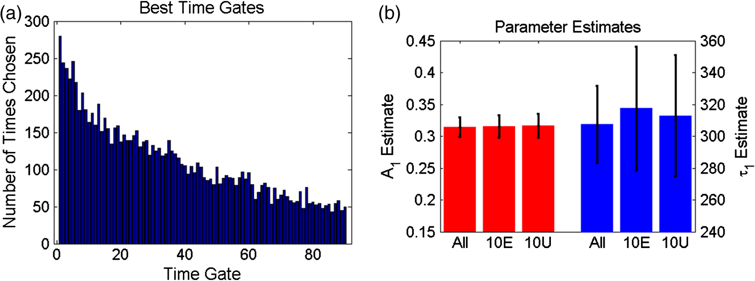

Second, the effect of the number of time gates on fitting accuracy was investigated using the same model parameters and with 1000 runs. The errors associated with the two estimated model parameters are provided in Fig. 4. For comparison, we provide both estimation errors for LSQR and RLD methods. As expected, at the nominal parameter values of $A_1=0.3$ and ${\tau }_1=300\mathrm{ps}$, the error increases as fewer time gates are considered, error being defined as the difference between simulated and mean of the estimations. The error between the estimate and model for $A_1$ was within 6% and for ${\tau }_1$ was within 4% (11 ps) in the case where all time gates are used. The error in the estimation of parameters when using full datasets can be attributed to the ill-posedness of the biexponential fits and Poisson noise. Similar levels of uncertainty are maintained using up to 10 gates for fitting. When reducing the number of time gates further, the errors increase up to 22% when using only four gates. A similar trend can be observed when focusing on the standard deviation for the error estimation, based on the 1000 trials. Hence, these results suggest that fitting with 10 equally spaced gates yields similar results as using full temporal datasets (90 gates). Note that RLD is generally unstable with a short lifetime of size similar to that of the IRF. The average error for $A_1$ was about 90%, and the average error for ${\tau }_1$ was 2% over 1000 runs, but with a standard deviation of more than 100 ps.

Fig. 4

Average and standard error associated with parameter estimation when using sparse temporal datasets and RLD for model parameters (a) $A_1$ and (b) ${\tau }_1$. The expected values are 0.3 and 300, respectively.

To assess if these findings were dependent on the model parameters, these error functions were estimated over a full functional range of values that can be encountered in biexponential applications. Results are given in Fig. 5. The trend is similar when the experiment is expanded across the entire parameter space. Average error in $A_1$ across all parameter combinations using all time gates was within 5% and increased to 19% (with local peak errors approaching 60%) using four time gates. Again, a large increase in the average error across all combinations occurs when the number of time gates is reduced from 10 (6%) to 6 (14%). For small fractional amplitudes ($A_1$ $\in$ [0.1 to 0.2]), the error in $A_1$ using six and four time gates significantly increases for all values of ${\tau }_1$, ranging from 40% to 60%. Overall, these simulations establish that using 10 time gates results in similar estimation accuracy as using full temporal data for the parameter range of ${\tau }_1$ $\in$ [250 to 450] ps and $A_1$ $\in$ [0.1 to 0.9]. The average error in estimating $A_1$ across the entire parameter space was increased by only 1% when sampling down the temporal data from 90 gates to 10 gates. A reduction in time-gate acquisition of this magnitude would result in almost a 10-fold decrease in acquisition time required, while yielding the same biological insights based on model parameters fitted.

Fig. 5

Percent error in $A_1$ estimation when using different numbers of gates (90, 45, 23, 10, six, and four) for ${\tau }_1$ $\in$ [250 to 450] ps and $A_1$ $\in$ [0.1 to 0.9].

3.2.

Validation In Vitro and In Vivo

In order to validate the results obtained from in silico simulations, the findings are applied to cell-based assay and in vivo experiments. Experimental results were originally acquired using 120 time gates, approximately 90 of which fall in the asymptotic part of the measurements. Parameter estimation is performed using the entire set of available time gates in addition to using reduced subsets of time gates. Of particular interest in each of these experimental procedures is $A_1$, the quenched donor fraction, which represents the fraction of Tfn bound donor that underwent cellular internalization. Data were acquired using wide-field excitation and acquisition, as described in Sec. 2.4. A comparison of estimation errors in $A_1$ for a subset of the data is made in Table 1 and Fig. 6. Table 1 shows a subset of the results for both cell lines compared with previous simulation results. The data agree well with the results from simulations with a similar trend occurring in all three datasets. In both cell lines, the error is approximately the same when using 90, 45, 23, or 10 time gates in addition to having similar standard deviations. Like the in silico experiments, there is also a large increase in error between using 10 and 6 time gates. Figure 6 shows the $A_1$ estimates from the T47D cell line across all AD ratios using several subsets of gates. Results using all or 10 time gates have similar mean estimates and standard deviations, whereas the results using four time gates tend to have larger standard deviations and different means. Note, however, that in all cases, the linear trend with increasing AD ratio is present and is similar to the result in Fig. 2(c).

Table 1

A subset of the A1 estimates (error % in parenthesis) using in vitro data and different sets of time gates compared with simulation results. In vitro data are from wells with an AD ratio of 0:1.

Fig. 6

Estimation of $A_1$ using in vitro experimental data (T47D cell line) and all, 10, or four time gates. The linear relationship in AD ratio is retained in all cases; however, using 10 time gates more accurately tracks the linear relationship.

In vivo data were collected as described in Sec. 2.5. The data were fitted using the complete (90) set of time gates as well as the reduced sets of 10 and four time gates. The quenched donor fraction ($A_1$) was estimated in the tumor of the mouse in addition to the bladder as shown in Fig. 7. The mean $A_1$ estimates in the tumor are greater than in the bladder using each set of time gates (cf. Table 2). In each case, using 10 time gates results in similar mean estimates and little or no difference in standard deviation compared with using 90 time gates. The means vary by an average of approximately 4%, but because there is no ground truth information available, the total difference in error is not measurable. Using four time gates results in a higher average difference in mean of approximately 7% in addition to a larger standard deviation compared with using 90 time gates. Note that these results are consistent with the expected physiological results. The tumor model employed herein overexpresses TfnR, whereas minimal FRET Tfn is expected in the bladder. Hence, it is expected that the tumor would exhibit a larger mean $A_1$ as higher values of $A_1$ represent a larger portion of Tfn on the endocytic pathway.

Fig. 7

Comparison of in vivo estimations of $A_1$ in the bladder and the tumor (larger circle) of a mouse using (a) all time gates, (b) 10 time gates, and (c) four time gates. The estimations have been overlaid on a bright field image to provide the context. Results are largely similar with the bladder having a lower average $A_1$ estimate than the tumor, as expected.

Table 2

A comparison of in vivo A1 estimates using different sets of time gates. Using 10 time gates to fit the data results in similar estimates with similar standard deviations to the case of using all time gates. Using four time gates results in larger standard deviations and less accurate estimations, especially in the tumor.

3.3.

Discussion

Overall, these results suggest that by reducing the total number of time gates acquired from 90 to 10, FLIM-FRET acquisition time can be reduced by approximately an order of magnitude without greatly sacrificing the estimation accuracy. This is a significant result, especially for in vitro and in vivo platforms where FLIM-FRET techniques have yet to be widely adopted because of lengthy imaging times. Imaging platforms designed for drug discovery applications have recently been described by Talbot et al.⁵³ and Alibhai et al.⁵⁴ to take 30 and 46 min., respectively, to acquire a 96-well plate. By applying the methods described herein, a 96-well plate could be imaged in less than 1 min. These short acquisition times are particularly attractive for high-throughput FRET assays. Not only will such a platform be able to greatly increase the number of wells imaged in one session, but it will also permit increased multiplexing to significantly increase the number of processes studied. This will prove critical in enabling the design and optimization of new therapies using in vitro FLIM-FRET platforms.

Moreover, we have recently demonstrated that our novel wide-field imaging FLIM-FRET approach offers the possibility to employ well-characterized quantitative metrics used in FRET microscopy, but with the additional benefit of a seamless technological platform to perform in vivo quantitative assays. Based on wide-field patterned time-resolved illumination and gated detection,⁵⁵ we demonstrated that it was possible to retrieve in 3-D the quantitative biodistribution of the quenched donor fraction within 5% of in vitro data. However, as multiple projections are required to resolve the depth information based on an optical inverse problem,^56–58 the imaging protocols typically take around 45 min for whole-body imaging. In comparison, current time-resolved tomography platforms typically are able to image only cross-sections (two dimensional) of the animal and require imaging acquisition times of between 30 and 45 min.^59,60 Similar to in vitro data, temporal data reduction can lead to reduced acquisition times. Based on the findings of this work, we expect to be able to perform the whole-body 3-D FLIM-FRET in live animals in less than 5 min. Such fast acquisition speed will enable investigation of locally resolved fast pharmacokinetics studies in vivo, imaging multiple FRET pairs sequentially in reasonable time frames, and an increase in overall imaging throughput. These developments will be critical to establish FLIM-FRET as a reliable and attractive quantitative assay to the biomedical community for in vivo applications.