
|
|
1.IntroductionIn the past 15 to 20 years, there has been an explosion in the advancement of imaging instrumentation and analytical tools to measure molecular dynamics in live cells. Diverse processes such as chemical kinetics, molecular diffusion, protein transport, protein oligomerization, molecular interactions, and stoichiometries can now be followed with single molecule sensitivity and at microsecond timescales in biological systems.1–18 These microscopy-based techniques that make up this burgeoning field at the interface of biology and physics are collectively called fluorescence fluctuation spectroscopy (FFS) techniques (for review, see Refs. 1920.–21). At the heart of FFS techniques lies the ability to extract molecular dynamic information, such as diffusion and size, through analysis of the fluctuations that occur in the fluorescent signal emitted from the molecule of interest (Fig. 1). In fluorescence correlation spectroscopy (FCS), the time-dependent variation in the fluorescent signal is analyzed using an autocorrelation function to determine diffusion rates and concentrations of molecular species.22,23 However, the size/hydrodynamic radius of a molecular species can be difficult to measure by FCS because the diffusion rate of a molecule is proportional to the cube root of its volume. This means that the size must increase about eightfold to detect a twofold increase in the diffusion rate.24 To circumvent this limitation, the complementary approach of photon-counting histogram (PCH) analysis, using the same dataset collected from FCS, was developed to extract the average number of fluorophores in the diffusing species.25,26 If the diffusing species are homogenous and do not contain unlabeled molecules, then the oligomerization state can be inferred by comparing the molecular brightness of the unknown species to a control (monomer or dimer). In PCH analysis, the photons of the fluorescent signal are counted to plot a histogram and the ratio of the signal fluctuations (variance) to average intensity is calculated to give the molecular brightness defined as counts per second per molecule (CPSM, Ref. 25). Therefore, the average fluorescent intensity of a 0.5-nM solution of a dimer (two fluorescent dyes) would have the same average intensity as 1 nM of a monomer (one fluorescent dye), but the molecular brightness of the dimer would be twice that of the monomer due to the larger variance. Fluorescence cross-correlation spectroscopy and dual-color PCH are FFS techniques used to measure the dynamics of two different fluorescently labeled molecules (e.g., green and red fluorophores) and are robust in detecting complex formation and dissociation events.19,20 The imaging extensions of FCS and PCH analyses are called raster image correlation spectroscopy (RICS) and number and brightness (N&B) analysis, respectively.21,27,28 RICS and N&B analyses allow for the spatiotemporal mapping of protein dynamics across an entire cell on microsecond to second time scales by exploiting the hidden time structure of the scanning laser beam of a confocal microscope. For example, examination of the spatial spread of the diffusion using RICS can help distinguish between simple diffusion and the binding/unbinding equilibria that can be more difficult to determine by spot measurements. Fig. 1Schematic illustrating four fluorescence fluctuation techniques (FFTs) used to measure protein dynamics in cells. Left: cartoon depiction of cell being imaged using a confocal microscope setup. fluorescent image of one-photon confocal volume with dotted line superimposed to represent the random diffusion of a fluorescently labeled molecule. Middle: fluorescent signal trace from a single fixed spot in the cell, or the laser beam can be raster scanned to record frames of images in the cell. Right: autocorrelation curves [fluorescence correlation spectroscopy (FCS)] from spot measurements can be fitted to obtain diffusion rates for the fluorescent molecules. The same dataset can be used to generate a photon-counting histogram (PCH) that can be fitted to obtain a molecular brightness. Diffusion [raster image correlation spectroscopy (RICS)] and molecular brightness [number and brightness (N&B)] values can be extracted from the raster scan images on a per pixel basis to generate spatiotemporal diffusion and molecular brightness maps, respectively. 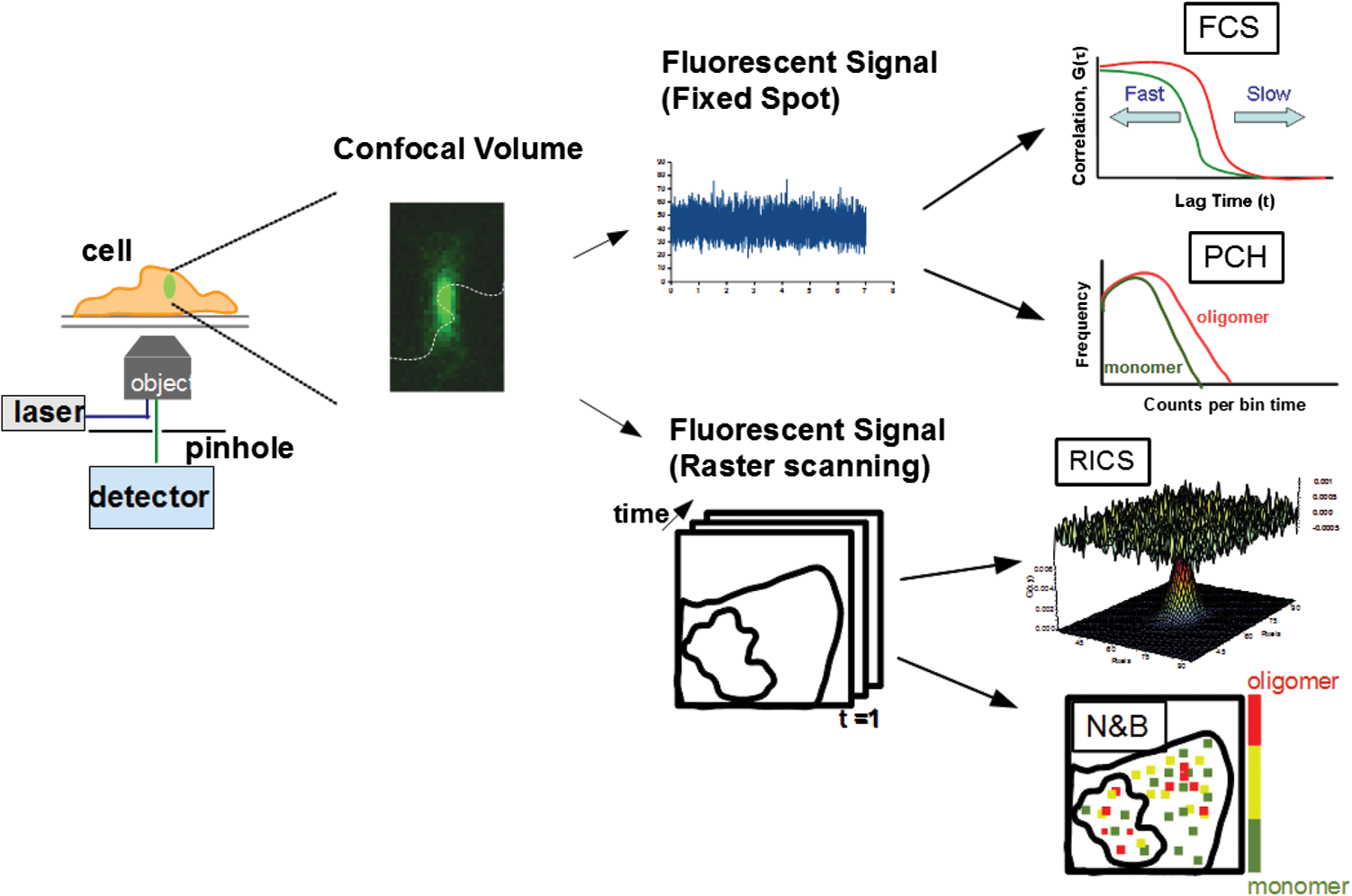 The molecular brightness can be ascertained by FCS, PCH, or N&B analysis if the data are properly acquired and normalized to control(s), thus yielding information about the stoichiometry of the diffusing specie(s). In fact, MacDonald and colleagues have shown that under optimal conditions, the brightness of AlexaFluor-488 dye is similar regardless of the techniques used.29 Importantly, FFS techniques rely on the statistical analysis of the fluctuations in the fluorescent signal to extract dynamic information about the diffusing species; any fluctuations not due to the molecular processes under investigation, such as system instabilities, will generate artifacts that complicate interpretations of the collected data. System instabilities that can contaminate the signal include fluctuations due to stage drift, sample movement, laser power variations, illumination volume geometry artifacts, undesired photophysics of fluorophore, and photobleaching of the fluorescence. Measurements of molecular brightness in living systems, such as eukaryotic cells, are not optimal due to a variety of diverse factors that include cellular movement, sample thickness bias, geometric constraints, and slow diffusion of molecules leading to a greater propensity for photobleaching.29–33 Are all brightness analysis techniques equivalent when studying protein dynamics inside complex living systems under nonideal conditions? The purpose of this tutorial is twofold: (1) provide practical advice for the implementation of three widely used FFS techniques (FCS, PCH, and N&B) in measuring the molecular brightness of proteins in live cells and (2) provide two examples where these techniques are not equivalent in determining molecular brightness due to system instabilities, properties of the protein under investigation, or the mode of acquisition (spot scan versus raster scan). 2.Theory of Fluorescence Fluctuation Spectroscopy TechniquesSeveral excellent reviews have been written describing the theory of FFS techniques and the reader is directed to these sources for an in-depth theoretical discussion.19–21,34–36 Summarized below are the basic principles and underlying statistical analyses used to extract molecular brightness values from fluorescence intensity measurements for FCS, PCH, and N&B methods. 2.1.FCS AnalysisThe basis of FCS analysis is that the fluorescent intensity is varying because molecules enter and leave the illumination volume over time due to Brownian or directed diffusion. For the FCS technique to work, the concentration of the molecules under investigation must be low, nanomolar to micromolar range, for the fluctuations not to be averaged out. This is trivial to achieve in vitro where the concentration of the molecules to be studied can be easily manipulated. This requirement for low concentrations of particles limited the use of FCS for biological measurements until the invention of the confocal microscope in the 1990s even though FCS has been employed since the late 1970s to study molecular dynamics in vitro.10,11,22,23 Today’s confocal microscopes can typically create a diffraction-limited spot (illumination volume) to if the pinhole is kept to Airy unit (AU) (Fig. 1, left panel). The change in the fluorescent intensity () at equilibrium is determined by subtracting the average intensity (brackets indicate average) from the signal intensity at a given time [Eq. (1)]: Comparison of to itself at different lag times () is called the autocorrelation function [], which is a measure of the similarity of the signal to itself over time [Eq. (2)]: Plotting the autocorrelation function [] versus time creates an FCS curve with a characteristic decay for the species being investigated (Fig. 1, right panel). The time corresponding to the half maximum of the fitted autocorrelation curve is the diffusion time of the molecule. Calibration of the waist of the illumination volume is needed to determine the diffusion rate and can be calculated by several different means, such as measurement of a fluorophore with a known diffusion coefficient or imaging of diffraction-limited beads (see Sec. 3.1). The inverse of the amplitude of the FCS curve at is equal to the average number of particles diffusing through the illumination volume but only if the number of fluctuations obey Poisson statistics. Therefore, the molecular brightness () of the diffusing species can be calculated by dividing the average count rate () by the average number of particles () recovered from the FCS curve fit (). Concentration measurements can also be made once the and volume have been determined, providing a robust way to measure concentration differences in cellular compartments. The relationship between the fluctuation intensity and the average number of particles in the illumination volume has been exploited by several groups to study protein dimerization and protein ligand interactions using the inverse relationship between the particle number and amplitude of the FCS curve (). In the case of dimerization, as the particle number drops to half because of complex formation, the fluctuation amplitude of the FCS curve () will double.37–41 This relationship holds true if the total protein concentration is stable during the FCS measurement. This method of using intensity (first moment) and variance (second moment) information from FCS measurements to calculate molecular brightness is termed moment analysis. Moment analysis is successful when applied to homogenous single species samples, but interpretation of the fluctuation amplitude is very difficult when there are multiple species of varying concentrations because molecular brightness contributes nonlinearly to the fluctuation amplitude.29,42 In addition, higher moments and a much larger dataset are required to adequately describe all species using moment analysis on FCS datasets.29 Therefore, the exact concentrations of the different species must be known to adequately describe the amplitude and , which is not always possible. For these reasons, complementary approaches to analyze fluctuation amplitudes for determination of molecular brightness and number information for multiple species were developed, such as PCH analysis. 2.2.RICS AnalysisIn FCS analysis, only signal fluctuations at one point of illumination are measured, but in RICS analysis, fluctuations from multiple volumes are considered both near (adjacent pixels) and far (nonadjacent pixels). This allows a more complete description of the probability of finding a diffusing particle in space and time. A single spot measurement would be sufficient to describe the isotropic diffusion of a particle because its movement is uniform in space and time. In contrast, RICS is better suited for the measurement of particles with anisotropic behavior (diffusion rate varying in space and time) compared to FCS. Importantly, the pixel dwell time and pixel size must be compatible with the particle diffusion being studied in order to perform RICS measurements. If the scan speed is too fast, then the particle will appear immobile, but if the speed is too slow, then the particle will diffuse away before being detected in subsequent pixels. Pixel sizes ranging from 0.025 to and pixel dwell times ranging from 2 to will be sufficient to measure the dynamics of a wide range of molecular species. For example, a pixel size of and dwell time of are sufficient for capturing the movement of a 25 kDa protein diffusing in the cytoplasm of a cell by pixel 2-3 of the scan.21,28 To prevent undersampling, a minimum region of interest (ROI) of is recommended by Brown and colleagues based on simulations and experimental measurements of enhanced green fluorescent protein (EGFP) in solution.43 The typical resolution of RICS is based on a 16-pixel subframe commonly used for analysis (16 pixels averaged; size) and is approximately two to three fold lower than FCS.21 Finally, cellular movement or immobile structures within cells can lead to artifacts in the correlation function and, therefore, a high-pass filter algorithm may be needed during image analysis. 2.3.PCH AnalysisThe amplitudes of the fluorescence signal can be analyzed by binning the data and plotting frequency as a function of photon counts per bin-time, which is called a PCH histogram plot. In this way, the entire photon distribution can be considered based on the first and second moments of the signal. A PCH plot of a single molecular species can be fully characterized by defining the average number of molecules per illumination volume and the photon counts per molecule per second (i.e., molecular brightness, ). The shape of the plot is influenced by the intensity heterogeneity of the point spread function (PSF), Poisson shot noise from the detector, and fluctuation in molecule numbers. Any fitting method must account for these variables to obtain an accurate molecular brightness. The histogram is fitted using a nonlinear least square fitting method, such as Levenberg-Marquardt or Gauss-Newton, to equation to obtain the variance (), where is the probability of the measured photon counts in a bin and is the total number of measurements. In the above-mentioned equation, intensity () and photon counts () are interchangeable under these circumstances, but is used because it pertains to fitting a PCH plot. The variance and average intensity of the signal are then inserted into Eq. (3) to calculate the molecular brightness of the molecule: where is the variance, is the intensity of the signal, represents the fractional intensity of species, and is the geometric shape of the PSF.42 If there are two molecular species in the sample, for example, the resultant histogram will be convolved to reflect the contributions from both species and the histogram can be fitted to obtain additional N&B parameters to account for the extra species. Additional analytical methods that use different mathematical approaches but are functionally equivalent to PCH analysis have been described but will not be discussed here and the reader is directed to Refs. 4445.–46 for more information. Finally, methods have been developed that allow the determination of brightness and diffusion information by combining the advantages of FCS and PCH.472.4.N&B AnalysisIt is cumbersome to perform FCS and PCH measurements on biological samples, such as eukaryotic cells, because only a single illumination volume in a selected location can be measured. Measuring the entire cell would take an inordinately long time, require a large number of observations per image pixel, and would be computationally slow. N&B analysis allows the extraction of average molecular brightness and numbers of particles from individual pixels of a raster scanned image using moment analysis.27 The method was originally developed to study the aggregation state of a protein subunit during assembly/disassembly of focal adhesion complexes.16 In N&B analysis, the average counts per integration time () and variance () at each pixel is calculated and the following two equations are used to calculate average apparent brightness [, Eq. (4)] and apparent number of particles [, Eq. (5)]: Variances from the fluorescent molecules (dim fast diffusing, bright slow diffusing, and immobile), autofluorescence, light scattering, and noises of the detector all contribute to the total signal variance. If these sources of variance are independent, the total variance is simply the sum of the individual variances. Fortunately, these variances do not have to be accounted for individually because only the mobile molecules/particle fluctuations vary with the square of the brightness () leading to a value .27 In contrast, immobile particles do not have fluorescence fluctuations so that the variance () in the pixel and the ratio of are zero and is 1. An increase of the illumination intensity can be used to confirm that the variance originates from the particles of interest because a plot of variance as a function of intensity should have a quadratic relationship. Subtraction of 1 from yields a true molecular brightness . This is necessary in order to remove the detector count statistics that contribute to the variance (for the mathematical basis, see Ref. 27). The true number of particles can be calculated using the following equation [Eq. (6)]. Again, this is necessary to correct for the noise contributed by the detector. It is important to select an appropriate pixel dwell time that is long enough to adequately sample the fluctuations but avoids averaging out the signal fluctuations. For example, a pixel dwell time of is reasonable if one is studying a protein diffusing inside a cell at . Photon-counting detectors are ideal for N&B measurements because the registered photon event correlates one-to-one with the signal generated unlike analog detector systems that record digital levels. However, analog systems can be used for N&B analysis as long as the average count rate () and values are corrected for the digital offset () and digital levels per photon (), respectively [Eqs. (7) and (8), Refs. 21 and 48]: Each time the voltage or gain is changed on the analog detector, the calibration must be repeated to determine the new value. Limitations to N&B analysis are that fast-moving particles, such as fluorescent dyes, in solution sometimes cannot be measured and the observation volume is roughly three fold larger in the plane compared to the volume for FCS/PCH measurements because of the raster scanning of the laser. Importantly, mixtures of multiple species with different brightnesses residing in the same pixel cannot be resolved by N&B analysis and only the weighted average brightnesses obtained.27 In contrast, the technique is robust for identifying spatially heterogeneous clusters of particles/species in an image.7,9,15,16,27 2.5.Summary of FFS TheoriesMolecular brightness determination using FCS data is well suited for homogenous single species, but this method breaks down in the face of more complex heterogeneous samples. In contrast, the PCH method for calculating molecular brightness takes the entire photon-count distribution into consideration and can be used to resolve samples containing multiple species of varying brightness. The recently developed technique of N&B analysis applies moment analysis to extract N&B information from individual pixels of a raster scanned image, making it amenable for measuring biological samples, such as cells. The molecular oligomerization measured by FFTs represents the minimum stoichiometries in systems where fluorescently labeled and unlabeled molecules coexist. Therefore, it is useful to perform experiments in the absence of unlabeled molecules when possible. Importantly, the brightness values obtained from all three measurements depend on the laser intensity employed. For example, higher laser powers will give rise to higher brightness values. The intrinsic characteristics of the detector, such as dead-time and afterpulsing, also affect the brightness values obtained. For these reasons, all measurements should be performed at the same detector and laser power settings. Routinely, relative brightness values are given instead of absolute values for comparison since different research groups have different experimental setups. 3.Calibration of Microscope for FFS Measurements3.1.Calibration of Detection VolumeWe recommend periodically checking the size and shape of the confocal volume (once every three months) to identify any deviations that could arise due to system damage/misalignment. Three commonly used methods to measure the shape and size of the confocal volume are (1) dilution series measurement of a dye with a known concentration, (2) measurement of a dye with a known diffusion coefficient, and (3) measurement from raster scanned images of the subresolution fluorescent bead. The advantages of the first method for volume determination are that the calibration and experiment can be performed under similar conditions and no information about the shape of the volume is needed. This is because the effective volume () can be calculated using (correlation amplitude), Avogadro’s number (Na), and the concentration of the solution () and without mathematical fitting of the FCS curve by using Eq. (9): The second method does not require knowledge of the solution’s concentration but only the known diffusion coefficient () for the fluorescent molecule. This method does assume the effective volume is Gaussian and the effective volume can be calculated using Eq. (10): Solving Eq. (10) is usually done with fixed and the other variables (, eccentricity/structural parameter = ratio of axial radius to lateral radius; ) obtained from the fitted FCS curve. Unlike the first two methods, the third method directly measures the confocal volume () using subresolution fluorescent beads as a point source and can be converted to the using Eq. (11): A bead size of 100 to 170 nm is suitable for calibration and the size will not impact the calibration as long as it is smaller than the diffraction-limited spot. There is a freely available ImageJ plugin that automates the analysis of the fluorescent bead image series that we have found quite helpful.49 All three methods yield comparable results and the bead scanning method is particularly fast when image analysis is automated using ImageJ. For a more in-depth discussion of volume calibration methods, see the PicoQuant application note.50 3.2.Determination of Detector SensitivityThe microscope detector sensitivity and optimal laser power must be determined before the molecular brightness of the sample can be measured. Measurement of either a purified fluorescent dye or fluorescent protein to be used in the experiment is a good choice for characterizing the microscope system. Since many of our experiments involve measuring the dynamics of GFP-tagged proteins in mammalian cells, we chose to use purified EGFP to characterize our one-photon Zeiss LSM 510 META ConfoCor 3 microscope system. The following calibration experiments are applicable to characterize all microscope systems equipped to perform FFT measurements. First, we measured different concentrations of purified EGFP in solution using a constant low laser power setting [0.45 μW at the sample level, 488 nm argon laser, Fig. 2(a)]. The molecular brightness was determined either from fitted FCS data by dividing the average count rate by the recovered particle number or from the fitted PCH curve. It is apparent that the molecular brightness of EGFP is stable from 20 to 160 nM and similar brightnesses are obtained whether FCS or PCH data are used (6123 and 6703 cpsm, respectively). However, brightness values became unstable at EGFP concentrations , falling to about half the average values at 2.5 nM [2825 cpsm (FCS) and 3994 cpsm (PCH)]. A similar trend was observed for EGFP brightness values measured by N&B analysis [20 to 160 nM, 3723 cpsm; 2.5 nM, 1385 cpsm, Fig. 2(b)]. The same laser power was used for FCS/PCH and N&B measurements, but the N&B values are lower because of the reduced laser exposure time, due to raster scanning, that the EGFP molecules experience as the laser scans across the sample. Based on these titration experiments, we set the lower sensitivity limit at 20 nM for our system [see dotted vertical line in Figs. 2(a) and 2(b)]. For our Zeiss microscope setup, we observed poor recovery of brightness values using FCS and PCH methods if our signal count rate dropped below 10 kHz even though our background signal for the buffer alone was . Fig. 2Characterization of microscope system detector sensitivity. The concentrations of the enhanced green fluorescent protein (EGFP) solution were varied from 2.5 to 160 nM. The laser power was attenuated to , at the sample level, of a 30-mW argon laser. (a) Plot of molecular brightness expressed as counts per second per molecule (CPSM) as a function of the EGFP concentration measured in vitro using either FCS (black squares) or PCH (gray diamonds) methods. (b) Plot of molecular brightness (CPSM) as a function of the EGFP concentrations based on N&B analysis. (c) and (d) Recovered diffusion coefficients as a function of the EGFP concentrations using FCS or RICS analysis, respectively. (e) and (f) Plot of EGFP concentration measured by spectrophotometer absorbance as a function of concentration measured by FCS or RICS analysis, respectively. Concentration calculated using effective (black squares) or confocal volume (orange diamonds) from 2.5, 5, 10, 20, 40, 80, and 160 nM EGFP solutions. Effective volume calculated using Eq. (9) and confocal volume determined from images of subresolution fluorescent beads using the equation . Data were collected on a Zeiss LSM 510-ConfoCor 3 equipped with avalanche photodiodes (APDs) and LD C-Apochromat water immersion objective. The laser was reflected by a dichroic mirror onto the sample and the emitted fluorescent signals were filtered with a 505- to 540-nm bandpass filter during acquisition. One hundred (50 nm pixel size) were acquired with pixel dwell time and 7.656 ms line time. Image analysis was performed using ZEN software (FCS/PCH) or SimFCS (RICS/N&B). 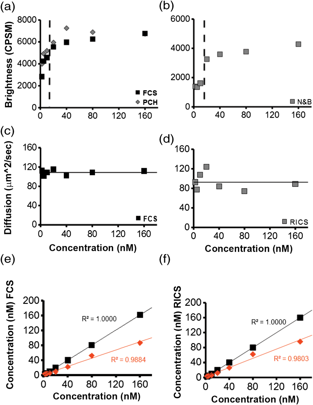 Both FCS and PCH analytical models assume that the confocal volume is three-dimensional (3-D) Gaussian and has no distortions. We acquired a 3-D image stack of a 0.17-micron AlexaFluor 488-labeled bead to confirm that our confocal volume has a Gaussian distribution in the and planes (Fig. 3). We also calculated the EGFP diffusion coefficient by using the FCS data or performing RICS on the image series as a second test to confirm that we had not saturated the illumination volume. The average diffusion rate obtained was 109 and for FCS and RICS, respectively [line in Figs. 2(c) and 2(d)]. These rates are in good agreement with the generally accepted rate of for EGFP in solution at room temperature.51 If the illumination volume had been saturated, we would expect the volume to be non-Gaussian and the equations used to fit the autocorrelation functions would return diffusion values significantly different from because the fitting equations assume a Gaussian observation volume. Fig. 3Representative point spread function (PSF) measurement to confirm Gaussian illumination intensity profile. (a) The intensity profile of the PSF measured from a fluorescent bead using a water immersion objective. PSF is derived from a Z-stack of 100 images ( frame with z-step of 200 nm, pixel size of 296 nm, pixel dwell time of and 1 Airy unit ), acquired on Zeiss LSM 510-ConfoCor 3. (b) The fitted curve (solid line) on the measured data points (open circles) demonstrating Gaussian profile with FWHM and FWHM dimensions giving a structural parameter of 2.93 and a confocal volume of 0.72 fl. All PSFs were generated and analyzed in ImageJ using the macro “MIPs for PSFs All Microscopes.”49  We plotted the recovered concentration of EGFP in solution as a function of nominal concentration (measured by absorbance) to determine the ability of FCS and RICS analyses to precisely measure concentrations [Figs. 2(e) and 2(f)]. Concentrations measured by both methods were determined using either the effective volume or confocal volume in the calculation. Concentration calculation using the effective volume returned values almost identical to the absorbance readings. In contrast, the concentrations calculated using the confocal volume, determined from fluorescent bead measurements, were very similar up to 80 nM and then deviated strongly at the highest EGFP concentration (160 nM). This underestimation of concentration above 100 nM for RICS has been reported previously.43 The underestimation of values could be due to one of several reasons: (1) differences in the method of volume measurement (solution versus bead attached to slide), (2) nonfluorescent or aggregated protein, (3) adsorption to the chamber surfaces over time, or (4) due to small deviations in Gaussian shape (less likely). Regardless of the exact reason for this underestimation, both FCS and RICS can reliably measure concentrations up to 100 nM (count rate ) using our microscope setup, similar to a previous report,43 and recovered values deviated by 20 to 50% at count rates . We conclude that a signal-to-noise ratio (SNR) of at least is required for our avalanche photodiode (APD) detectors, concentrations up to 100 nM can be reliably measured, and the proper SNR and sensitivity should be determined for your microscope system. 3.3.Determination of Optimal Laser Power RangeWe chose the lower sensitivity limit (20 nM) to conduct power series experiments in order to determine an optimal laser setting for FFS measurements. Brightness values recovered by FCS and PCH methods plateaued at laser power. There was a sharp decline in brightness values at laser settings , indicating saturation of the illumination volume [Fig. 4(a)]. This saturation was confirmed by an initial rise and then a sharp decline in recovered diffusion coefficients as laser power was increased from 8.1 to (at the sample level) due to photodynamic processes [bleaching and flickering, Fig. 4(c)]. From 0.45 to , the brightnesses increased linearly and FCS measurements should be kept in this linear range, preferably at the lowest setting possible. The maximum laser attenuation setting for FCS and PCH methods is for our microscope setup [dotted vertical line, Figs. 4(a) and 4(c)]. In contrast, the N&B method has a greater dynamic range with a linear increase in brightness values recovered from 0.45 to [Fig. 4(b)]. This observation is confirmed by the stable diffusion coefficients recovered across the entire range of power settings tested [Fig. 4(d)]. The upper power limit for measurements could be lower inside cells, but it is not always practical to do power series measurements inside cells due to the multiple variables that could affect the brightnesses. A rule of thumb is to determine the upper laser power setting in a defined environment, such as using purified components in vitro, and then set the laser power to 1/10 the limit for experiments. The upper limit in our case was , therefore, we chose to set the laser attenuation to ( the limit) for our cellular measurements. In most circumstances, this conservative setting will prevent illumination volume saturation and photobleaching during measurements. For molecules with very slow diffusion rates (e.g., membrane proteins), the laser power should be scaled to the residence time () in the detection volume because the “1/10” rule may not be sufficient to prevent bleaching. This can be difficult to do when the sample is very heterogeneous because of multiple species that have different diffusion rates, but scaling power based on diffusion should be done whenever feasible. Importantly, the same laser power must be used in order to compare brightness measurements between samples. In our experience, 0.45 to laser attenuation settings work reasonably well for measuring the dynamics of many cellular proteins. For our system, setting the attenuation usually results in unreliable power output. Fig. 4Determination of optimal laser power for FFT measurements. The laser power was varied from 0.45 to at the sample level of the 30-mW argon laser. The EGFP solution was set at 20 nM. (a) Plot of molecular brightness as a function of the laser power, measured using either FCS (black squares) or PCH (gray diamonds) methods. (b) Plot of molecular brightness as a function of the laser power based on N&B analysis. (c) and (d) Recovered diffusion coefficients as a function of laser power using FCS or RICS analysis, respectively. All Zeiss LSM 510-ConfoCor 3 settings are the same as in Fig. 2 with the exception of the laser power.  FFS measurements can be performed on experimental samples once the detector sensitivity, illumination volume shape, and power range have been determined for your microscope system. It is also important to be vigilant for system instabilities, such as stage drift due to thermal variations, or mechanical or optical misalignments. Other sources of variation that can lead to artifacts in measurements are cellular movements, photobleaching of slowly moving molecules, and sample thickness bias (see Sec. 3.4). 3.4.Discrepancy Between Brightness Values Measured In VivoRecent in vitro and in vivo studies have concluded that calculation of molecular brightnesses using FCS, PCH, and other single point FFS measurements are equivalent.5,6,29 However, photobleaching was observed in the studies performed on membrane proteins in cells, which could lead to an underestimation of the molecular brightness.5,6 Photobleaching is common for membrane proteins even when the laser power is carefully controlled because of the slow diffusion (1 to ) and the confinement to a two-dimensional (2-D) membrane. We performed measurements on a cytosolic protein (EGFP), a subunit of focal adhesion complexes (Paxillin), and a membrane-associated protein [EGFP-glycosylphosphatidylinositol (GPI)] to determine if brightness values obtained from different methods are indeed equivalent in vivo. HeLa cells expressing low levels of EGFP, EGFP-Paxillin, and EGFP-GPI were used for brightness measurements [Figs. 5(a1), 5(b1), and 5(c1)]. We define low levels of expression as cells having count rates of 150 kHz or below corresponding to nanomolar-to-micromolar concentrations. A z-scan was performed to position the illumination volume in the center of the fluorescently labeled cellular structure or cellular membrane depending on the protein being measured. Ten scans of 10 s were performed for each protein and the FCS/PCH curves were fitted (see protocols 1 and 2 for FCS and PCH). After FCS and PCH data collection, a stack of 100 images were collected for N&B analysis (see protocol 3 for N&B). The FCS and PCH experimental data fit well to a single component model as seen by the tight distribution of residuals [Figs. 5(a2), 5(b2), and 5(c2)]. The molecular brightness values for cytoplasmic EGFP were similar regardless of the method used [3730, FCS; 5309, PCH; 3920, N&B Fig. 5(a3)] or the microscope system used [4145, Leica TCS SP5 (data not shown)]. We also routinely measure the brightness of a tandem-EGFP protein (EGFP-linker-EGFP) to calibrate our brightness scale and the brightness is roughly twice that of EGFP, confirming the precision of our experimental setup (data not shown). Fig. 5Discrepancy between molecular brightness values for FCS, PCH, and N&B analyses in cells expressing EGFP-Paxillin or EGFP-glycosylphosphatidylinositol (GPI). (a1), (b1), and (c1) Fluorescence images of HeLa cells expressing EGFP, Paxillin-EGFP, or EGFP-GPI; (EGFP), (Paxillin-EGFP, EGFP-GPI). Crosshair indicates position of FCS/PCH measurement. Molecular brightness B maps were generated in SimFCS software. (a2), (b2), and (c2) Representative FCS curve and PCH histogram for EGFP, Paxillin-EGFP, or EGFP-GPI. The raw data are plotted in pink and the fitted curve is black with corresponding residuals below. FCS correlation curves were averaged from several 10-s scans to obtain better statistics. Bin time was 50 μs for PCH data analysis. Data were collected on the Zeiss LSM 510 META ConfoCor 3 system. (a3), (b3), (c3) Cytosolic EGFP molecular brightness is plotted as CPSM measured by FCS ( cells), PCH ( cells), and N&B analysis ( cells). Paxillin-EGFP molecular brightness is plotted as CPSM measured by FCS ( cells), PCH ( cells), and N&B analysis ( cells). EGFP-GPI molecular brightness is plotted as CPSM measured by FCS ( cells), PCH ( cells), and N&B analysis ( cells). Unpaired test, * (N&B versus PCH), * (N&B versus FCS). Errors are standard deviation. FCS, PCH, and N&B data are pooled from two experiments and analyzed using ZEN software (FCS/PCH) or SimFCS (N&B). 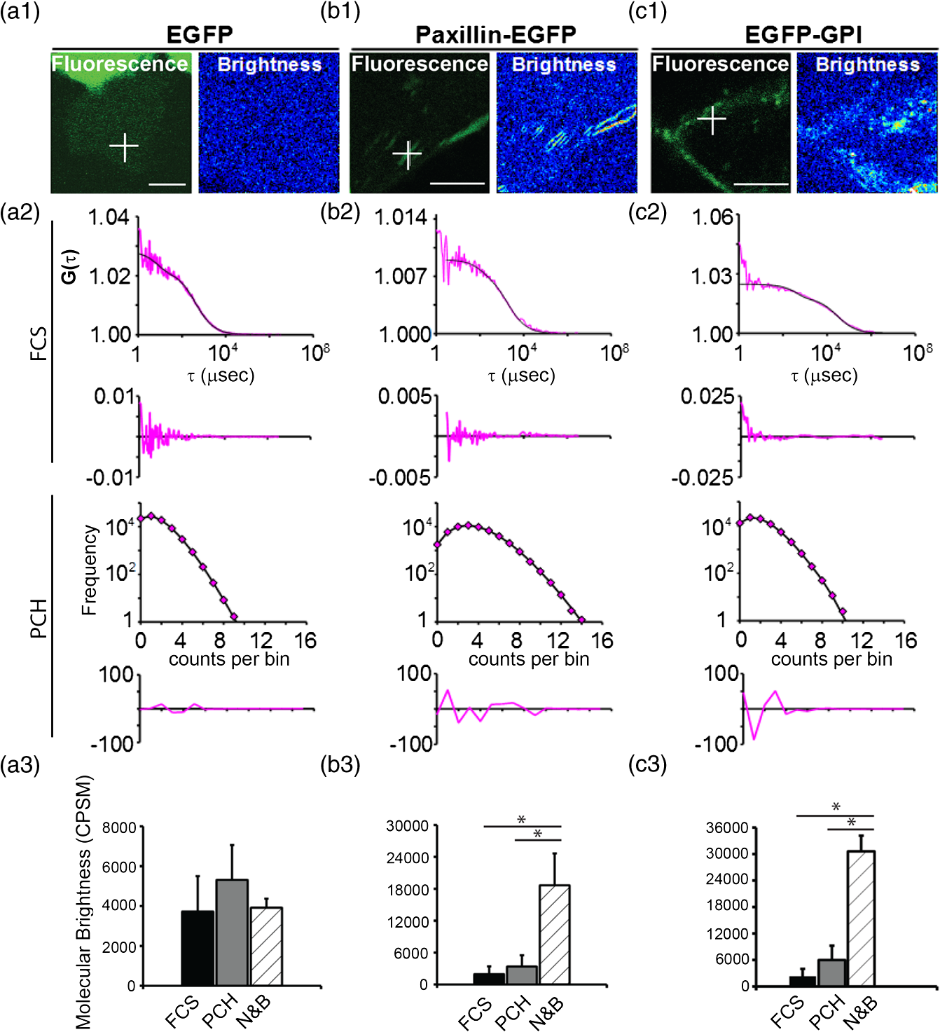 In contrast, there was a discrepancy in the brightness measurements for EGFP-Paxillin and EGFP-GPI. The average N&B brightness value for EGFP-Paxillin was 18,664 cpsm compared to and for FCS and PCH measurements, respectively [Fig. 5(b3)]. If we normalize our N&B brightness values, then we obtain an average of Paxillin molecules (range 2.9 to 9.3) dissociating from adhesions, which is in good agreement with previous N&B studies that found complexes ranging in size from 6 to 10 molecules.16 We also observed a discrepancy if we measure the brightness of the membrane anchored protein EGFP-GPI using FCS and PCH, versus N&B analysis [2287, FCS; 5978, PCH; 30,602, N&B Fig. 5(c3)]. The EGFP-GPI brightness values obtained by N&B analysis correspond to roughly five to eight molecules per cluster, which is similar to a recent study investigating the clustering of EGFP-GPI in a cell model of Fabry disease.52 We believe one reason for this discrepancy between the spot measurements (stationary laser beam) and the raster scanning approach is due to more photobleaching in the 10-s illumination time on a fixed spot versus dwell time on a pixel of an image frame. For both EGFP-Paxillin and EGFP-GPI, during several measurements, there was apparent photobleaching that occurred during the first 10-s scan that most likely represents slow-moving complexes being bleached (Fig. 6). Elegant studies using a combination of scanning FCS (sFCS) and RICS identified a heterogeneous dynamic behavior for Paxillin in cells.53 Based on these studies, monomers of Paxillin are thought to bind to quasi-immobile structures during adhesion assembly and large aggregates are released during disassembly.53 In the study, Digman et al. used a two-component model to fit their data. Fitting our PCH data for EGFP-Paxillin to a two-component model did not yield a better fit (data not shown). Fig. 6Photobleaching is partially responsible for underestimation of molecular brightness values for EGFP-Paxillin and EGFP-GPI using FCS/PCH methods. A representative photon count trace, measured with FCS, from EGFP in cytoplasm (a), EGFP-Paxillin in focal adhesions (b), and EGFP-GPI in plasma membrane (c). First trace of 10 shown. Note the photobleaching that was seen in a majority of cells expressing EGFP-Paxillin and EGFP-GPI measured but not EGFP. The photobleaching was seen in the first scan but not in subsequent scans and most likely represents bleaching of slowly moving large oligomeric species that can be detected by N&B analysis (see Fig. 5). Traces are fitted with trend lines to illustrate the decay of the intensity trace for EGFP-Paxillin and EGFP-GPI but not for EGFP.  This bleaching of EGFP-GPI during our FCS measurements has been observed by others.54 It is apparent that the bleaching subsides by the end of the scan and, indeed, subsequent scans2–10 are free of bleaching artifacts and these scans were used for analysis. The subsidence of the bleaching is most likely due to the complete bleaching of slow-moving/immobile species. In some instances, a visible bleached spot can be seen after acquisition. For our analysis, we left out the first scan and we believe this is leading to the underestimation of the molecular brightness for EGFP-Paxillin and EGFP-GPI using FCS/PCH methods because the large bleached species appear to be invisible during subsequent scans and are not replenished during the acquisition time frame. It is possible to correct for photobleaching and this has been accomplished in some instances.55,56 However, the full nature of the photobleaching must be characterized in order to correct for it, which is not always trivial. Paxillin clusters were detected using sFCS where the laser beam is moved across the sample, thus minimizing bleaching.53 Molecular brightness can become artificially inflated when the cell thickness falls below a critical value (; Ref. 29). This occurs because most mathematical models used to fit FFS data assume a finite uniform geometry that becomes confined and distorted as the sample thickness decreases due to a higher density of fluorescent molecules occupying the center of the volume. We were careful to choose cell areas for a measurement that were not too thin (), therefore, this is an unlikely reason for the discrepancy in brightness values. Regardless of the exact reasons for the discrepancy, it is clear that relying on one brightness method to determine oligomeric status of a protein from brightness measurements is not optimal, especially if photobleaching cannot be accurately corrected. 3.5.Summary and RecommendationsIn this tutorial, we review several different methods for determining molecular brightness values for fluorescent molecules. The basic theory for FFS measurements is provided along with the advantages and disadvantages of the particular methods. It is critical to properly calibrate and characterize your microscope system before performing actual experiments. We suggest performing concentration and laser power series experiments to determine the lower sensitivity limit and the optimal laser power, respectively. It is also important to characterize the shape of the illumination volume since the mathematical models for FFS techniques assume 3-D Gaussian profiles. If the volume is not 3-D Gaussian due to sample bias, the models can be modified to accommodate the altered shape.29 Performing this shape check is also valuable for confirming that the instrument optics are properly aligned and free of damage. Oil-immersion objectives have focal-depth dependences that can lead to distorted brightness values. Therefore, we recommend using water-immersion objectives that have a collar to correct for coverglass thickness and do not have depth distortions. Detector characteristics, such as deadtime and afterpulsing, can impact measurements, but this can be minimized if the signal intensities are kept well below saturation levels ( to ) and the fluctuations being studied are not on the same time scale as the detector traits. Detector deadtime and afterpulsing have to be corrected if fast chemical processes are being studied. Similar brightness values can be recovered independent of the FFS method used for well-defined systems in vitro.29 However, we demonstrate that for heterogeneous systems in vivo, this is not always true. The discrepancy in brightness values between methods can be partly linked to photobleaching of a subpopulation of the molecules due to the slower diffusion kinetics. Therefore, caution should be exercised when using only one brightness technique to infer the oligomeric status of a protein in cells and we argue, similar to several groups,29,53 that several complementary techniques should be employed and compared. Table 1 lists our recommendations for instrumentation requirements/settings based on our experience using a Zeiss LSM microscope system and can be used as a reference for other microscope systems. It is important to select cells expressing as low a fluorescent signal as possible but still maintaining a good SNR (e.g., ) for FFS measurements. We provide general protocols to perform FCS and PCH measurements that can be used with commercial or home-built microscope systems. We also provide a protocol for N&B analysis employing the SimFCS software that can be used with data collected from commercial confocal microscopes (e.g., Zeiss, Leica). Table 1Recommended equipment and settings for fluorescence fluctuation spectroscopy measurements.
Note: EGFP, enhanced green fluorescent protein. FFS techniques are robust and sensitive when the microscope system is properly calibrated and aligned. Importantly, care should be taken when interpreting FFS data for membrane or membrane-associated proteins in living cells due to the increased possibility of photobleaching and, thus, incorrect estimation of recovered parameters, such as molecular brightness. We hope that this tutorial containing practical advice and protocols will be of use to those routinely using FFS techniques and the wider scientific community, especially those persons interested in implementing these powerful techniques in their own laboratories. Protocol 1—FCS Protocol to Measure EGFP in Solution or Mammalian CellsMaterialsReagents
Equipment
ProcedureReagent setup
Equipment setup
Measure EGFP in Solution
Coverglass thickness measurement
Fig. 7Line scan mode window in Zeiss ZEN software (version 2008). (a) Intensity plotted as a function of pixel distance for reflected light from the bottom surface of a live cell dish. (b) Intensity plot from (a) after focusing on the coverglass bottom of the dish. Note the jump in the intensity line. From this point, moving the objective up lowers the line, and then the line jumps the second time (not shown here). The distance between the jumps of the line scan can be used to measure coverglass thickness.  FCS measurement for sample in solution
See Sec. 4.4 for details on how to fit data to obtain diffusion coefficient and how to calibrate volume. Measurement of EGFP Expressed in Mammalian Cells
Fig. 9Representative confocal image of EGFP expressing cell. (a) HeLa cell expressing low levels of EGFP amenable for FCS measurements surrounded by high expressing cells. Dotted line depicts boundary of the cell. (b) Zoom in the cytoplasm of the cell. Crosshair indicates where FCS spot measurement was made.  Note: Acquisition settingsThe scan time should be at least 1000 times longer than the diffusion time () of the molecule under investigation. For proteins expression in the cytoplasm, 10 s is usually sufficient. For membrane proteins, longer scan times, such as 25 to 100 s, are needed. For statistical purposes, performing one long scan is better than several shorter scans (e.g., versus ) because it improves the SNR. This is not always achievable when making measurements inside cells due to photobleaching. Usually, a compromise is made where 7 to 10 scans of 10 to 25 s are performed. Averaging these scans together gives statistics similar to one long scan. If photobleaching is a problem, then reduce the measurement time and increase repetitions. If the signal is too strong (e.g., ), then a preacquisition photobleach of the selected region can be performed. Note: Choice of fluorescent probesIf a fluorescent protein or dye other than EGFP is used, then change the dichroic mirror and filters accordingly. It is also important to make sure the probe does not have a high triplet state fraction under the laser excitation conditions used. There is no consensus in the field and acceptable levels of triplet formation range from to no . The levels of triplet species should be kept as low as possible. The probe should also be bright and resistant to photobleaching. However, no fluorescent probe has all the desirable characteristics and compromises are sometimes made. FCS Analysis
Fig. 8Example FCS and PCH data for GFP in solution. (a) Window in Zeiss ZEN software showing count rate plot, autocorrelation curve, and PCH for 30-nM GFP in solution. (b) Autocorrelation curve after removal of time points due to afterplusing.  For additional information, see Ref. 54. Protocol 2—PCH Analysis from Collected FCS DataCollection and Analysis of PCH Data
Fig. 10Options and Open File windows in Unruh ImageJ plugin. (a) The sampling frequency, PSF type, and file type can be selected in the Options window. In this example, the ConfoCor3 raw file type is selected. (b) Single or multiple files (highlighted) can be opened in the plugin.  Fig. 11PCH analysis and Fit Parameter windows in Unruh ImageJ plugin. (a) PCH analysis window displaying intensity (), brightness (), number (), and chi squared () for selected files. Red arrow points to the average value for all scans. Buttons on the right side allow for average, or global fitting and resetting fit parameters. (b) Selected curve window showing the PCH plot for the average of all the scans. Buttons on bottom allow for List, Save, Copy, Edit, and Select for plot. (c) Fit Parameter window showing variables that can be set for fitting or fixed value. (d) Average PCH plot after fitting to one species model. The fitted data (blue line) is directly over top of the data points (black line).  Protocol 3—N&B Image Collection and Data AnalysisAcquisition of Image Series for N&B Analysis(Note, > means open window in program. Image series acquired with the settings in this protocol can be used for both RICS and N&B analyses.)
Fig. 12Light Path window for Zeiss ZEN (version 2008). The dichroic mirror (HFT488/561) and bandpass filter (BP500-550) have been set for EGFP. A check mark indicates Ch2 (PMT) detector is active and the optical path is highlighted in white. An orange box has been added to direct the viewer to the relevant light path parameters. These parameters are used when searching for cells suitable for N&B/RICS acquisition. 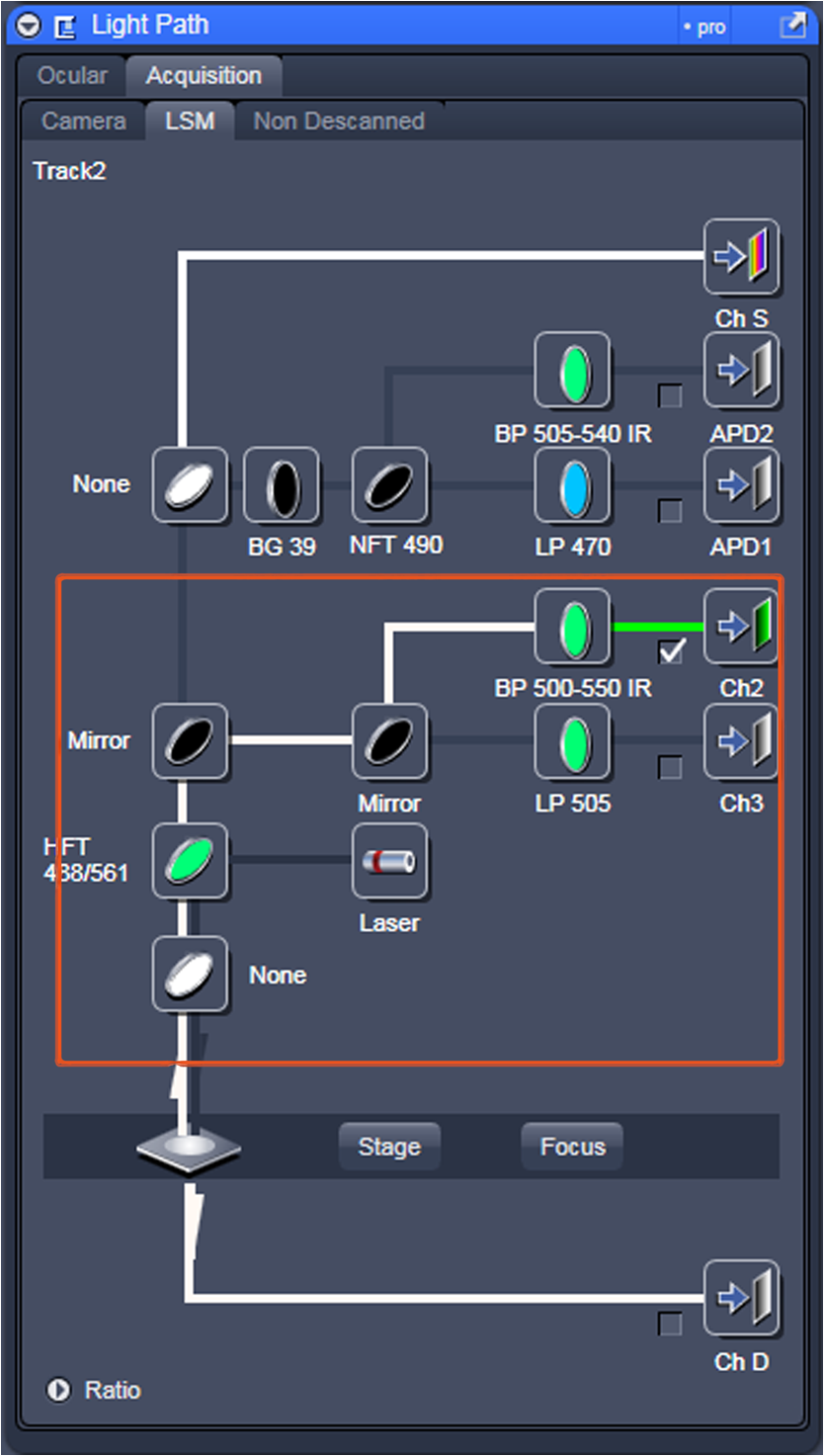 Fig. 13Light Path and Dyes window for Leica TCS SP5. The filter set for Alexa488 is selected (suitable for EGFP) and the light path is highlighted in yellow. The 488-nm line of the argon laser is set to 10% attenuation and the hybrid detector (HyD2) is set in standard mode. These settings are used when searching for cells suitable for N&B/RICS acquisition.  Fig. 14Acquisition window settings for Zeiss ZEN (version 2008) software for N&B. (a) ZEN acquisition window with the following settings used to collect N&B data: detector set to Ch2 (PMT), , , , (), , , , , and . (b) Fluorescent image of EGFP expressing HeLa cells—using settings in Fig. 14(a)—with cross-hair on low expressing cell (zoom ). (c) High zoom (17.5) of region selected by cross-hair for N&B/RICS acquisition from (b).  Fig. 15Acquisition window settings for Leica TCS SP5 software during data acquisition for N&B. Leica acquisition window with the following settings used to collect N&B data: acquisition , , , , . Make sure to check minimize to remove time delay between frame acquisitions.  Fig. 16Light Path window for Zeiss ZEN (version 2008) software for N&B. Same dichroic and bandpass filters as in Fig. 12 are used except that the APD detector is used here. An orange box has been added to direct the viewer to the relevant light path parameters.  Fig. 17Light Path window for Leica TCS SP5 software for N&B. Same settings as in Fig. 13 except that the laser is attenuated to 2% and the HyD2 detector is changed from standard to photon-counting mode. 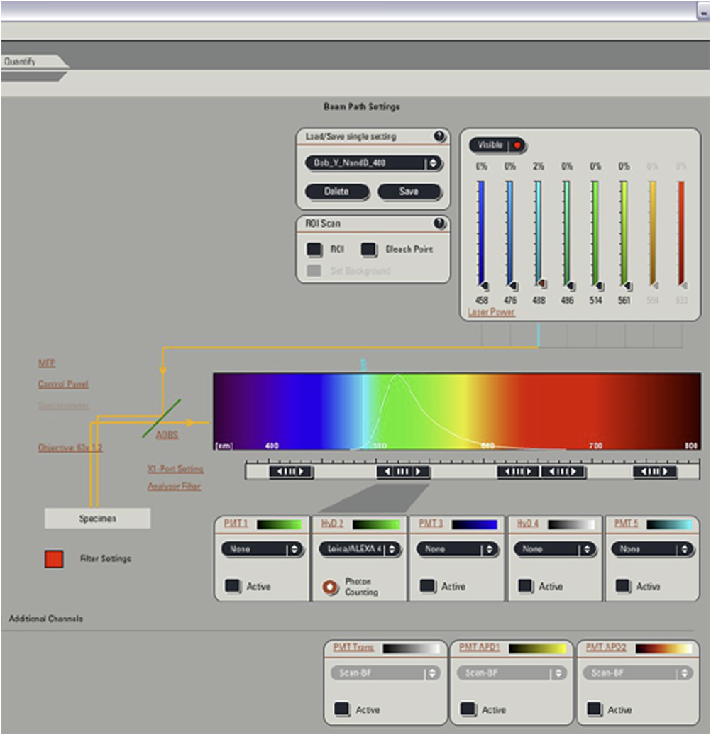 N&B Analysis Using SimFCS Software
Fig. 18SimFCS 2.0 Start and File Open windows. (a) Three analysis options (RICS, FLIM, SimFCS) are available upon starting the SimFCS program. The red arrow points to RICS button, which should be selected to start the N&B analysis. (b) Under File select Open Multiple Images (red arrow) to navigate to the folder where your image stack is located. Note: Figures 19 to 27 are all displays/windows in the SimFCS 2.0 software.  Fig. 19Main window. In the left image, one of the time series is displayed. To scroll through the stack of images, press the arrow button on image 1 frame (top red arrow). Scroll through the images and delete any images with obvious acquisition artifacts (due to stage drift, cell movement, etc.) (lower red arrow). Make sure to check the Use moving average to filter out slow cellular movement that can cause artifacts.  Fig. 20Tools menu. Select N and B option and Detrend (red arrow) to start the N&B analysis on the image series.  Fig. 21Analysis window. The upper left panel displays the brightness value () as a function of intensity, which we refer to as the B map (red arrow). Next to the B map panel is the selection panel. The far right series of panels displays histograms for average intensity, brightness (), and number (). Note: Subtract 1 in order to convert the brightness value to the molecular brightness ().  Fig. 22value correction when employing moving average filter. Select the Cal tab (red arrow) under the selection panel and input the value (red box) and then press the Recalculate N&B button (red asterisk).  Fig. 23Use of the spatial filter to sharpen B map. To bin the pixels and sharpen the B map, select the Filters tab and press the Smooth button (red box) once. The smooth filter can be used more than once, but there can be a loss of resolution. For comparison of different samples, it is best to smooth to the same extent.  Fig. 24Math tab in N&B window. Selecting the Math tab displays the average intensity, average variance, variance/intensity, true , and true for the entire image. Regions of interest (ROIs) can be created to calculate the value of that particular region (see Fig. 25).  Fig. 25Selection of ROI in N&B window. Under Cursors tab, select an ROI by clicking on the On box to the left size. The size of the ROI can be controlled by toggling the or value up and down. The ROI shape can be set as a circle or rectangle. Once the ROI is selected, the box will appear on the B map panel and can be moved around with the mouse cursor. The red arrow points to the location where the B value is displayed for the ROI.  Fig. 26Representative B map for EGFP in cytoplasm. Left: B map for EGFP expressed in a cell with the pixels corresponding to EGFP in the cytoplasm (red rectangle), background outside the cell (green rectangle), and an artifact (red circle). Right: arrows point to the corresponding pixels in the B value histogram. Note that the number of artificially bright pixels is a fraction (80) of the total pixels ().  AcknowledgmentsWe thank Michelle Digman for the Paxillin-enhanced green fluorescent protein plasmid and Venkatesan Raghavan for proofreading and helpful comments. R.T.Y. is grateful for support from the American Heart Association (12SDG8960000) and for imaging support from the Pittsburgh Center for Kidney Research (P30-DK079307). H.T. is supported from the NIH Technology Center for Network and Pathways grant 8U54GM103529 and is grateful for the Shared Imaging Facility at MBIC of Carnegie Mellon University. ReferencesK. BaciaI. V. MajoulP. Schwille,
“Probing the endocytic pathway in live cells using dual-color fluorescence cross-correlation analysis,”
Biophys. J., 83
(2), 1184
–1193
(2002). http://dx.doi.org/10.1016/S0006-3495(02)75242-9 BIOJAU 0006-3495 Google Scholar
E. Adu-Gyamfiet al.,
“Investigation of Ebola VP40 assembly and oligomerization in live cells using number and brightness analysis,”
Biophys. J., 102
(11), 2517
–2525
(2012). http://dx.doi.org/10.1016/j.bpj.2012.04.022 BIOJAU 0006-3495 Google Scholar
K. Baciaet al.,
“Fluorescence correlation spectroscopy relates rafts in model and native membranes,”
Biophys. J., 87
(2), 1034
–1043
(2004). http://dx.doi.org/10.1529/biophysj.104.040519 BIOJAU 0006-3495 Google Scholar
E. HausteinP. Schwille,
“Ultrasensitive investigations of biological systems by fluorescence correlation spectroscopy,”
Methods, 29
(2), 153
–166
(2003). http://dx.doi.org/10.1016/S1046-2023(02)00306-7 MTHDE9 1046-2023 Google Scholar
K. Herrick-Daviset al.,
“Fluorescence correlation spectroscopy analysis of serotonin, adrenergic, muscarinic, and dopamine receptor dimerization: the oligomer number puzzle,”
Mol. Pharmacol., 84
(4), 630
–642
(2013). http://dx.doi.org/10.1124/mol.113.087072 MOPMA3 0026-895X Google Scholar
K. Herrick-Daviset al.,
“Oligomer size of the serotonin 5-hydroxytryptamine 2C (5-HT2C) receptor revealed by fluorescence correlation spectroscopy with photon counting histogram analysis: evidence for homodimers without monomers or tetramers,”
J. Biol. Chem., 287
(28), 23604
–23614
(2012). http://dx.doi.org/10.1074/jbc.M112.350249 JBCHA3 0021-9258 Google Scholar
N. G. Jameset al.,
“Number and brightness analysis of LRRK2 oligomerization in live cells,”
Biophys. J., 102
(11), L41
–43
(2012). http://dx.doi.org/10.1016/j.bpj.2012.04.046 BIOJAU 0006-3495 Google Scholar
J. D. MullerY. ChenE. Gratton,
“Resolving heterogeneity on the single molecular level with the photon-counting histogram,”
Biophys. J., 78
(1), 474
–486
(2000). http://dx.doi.org/10.1016/S0006-3495(00)76610-0 BIOJAU 0006-3495 Google Scholar
G. Ossatoet al.,
“A two-step path to inclusion formation of huntingtin peptides revealed by number and brightness analysis,”
Biophys. J., 98
(12), 3078
–3085
(2010). http://dx.doi.org/10.1016/j.bpj.2010.02.058 BIOJAU 0006-3495 Google Scholar
P. Schwilleet al.,
“Molecular dynamics in living cells observed by fluorescence correlation spectroscopy with one- and two-photon excitation,”
Biophys. J., 77
(4), 2251
–2265
(1999). http://dx.doi.org/10.1016/S0006-3495(99)77065-7 BIOJAU 0006-3495 Google Scholar
P. SchwilleJ. KorlachW. W. Webb,
“Fluorescence correlation spectroscopy with single-molecule sensitivity on cell and model membranes,”
Cytometry, 36
(3), 176
–182
(1999). http://dx.doi.org/10.1002/(ISSN)1097-0320 CYTODQ 0196-4763 Google Scholar
P. Schwilleet al.,
“Fluorescence correlation spectroscopy reveals fast optical excitation-driven intramolecular dynamics of yellow fluorescent proteins,”
Proc. Natl. Acad. Sci. U. S. A., 97
(1), 151
–156
(2000). http://dx.doi.org/10.1073/pnas.97.1.151 PNASA6 0027-8424 Google Scholar
B. D. Slaughteret al.,
“SAM domain-based protein oligomerization observed by live-cell fluorescence fluctuation spectroscopy,”
PLoS One, 3
(4), e1931
(2008). http://dx.doi.org/10.1371/journal.pone.0001931 1932-6203 Google Scholar
B. D. SlaughterJ. W. SchwartzR. Li,
“Mapping dynamic protein interactions in MAP kinase signaling using live-cell fluorescence fluctuation spectroscopy and imaging,”
Proc. Natl. Acad. Sci. U. S. A., 104
(51), 20320
–20325
(2007). http://dx.doi.org/10.1073/pnas.0710336105 PNASA6 0027-8424 Google Scholar
R. T. Youkeret al.,
“Multiple motifs regulate apical sorting of p75 via a mechanism that involves dimerization and higher-order oligomerization,”
Mol. Biol. Cell, 24
(12), 1996
–2007
(2013). http://dx.doi.org/10.1091/mbc.E13-02-0078 MBCEEV 1059-1524 Google Scholar
M. A. Digmanet al.,
“Stoichiometry of molecular complexes at adhesions in living cells,”
Proc. Natl. Acad. Sci. U. S. A., 106
(7), 2170
–2175
(2009). http://dx.doi.org/10.1073/pnas.0806036106 PNASA6 0027-8424 Google Scholar
J. L. Swiftet al.,
“Quantification of receptor tyrosine kinase transactivation through direct dimerization and surface density measurements in single cells,”
Proc. Natl. Acad. Sci. U. S. A., 108
(17), 7016
–7021
(2011). http://dx.doi.org/10.1073/pnas.1018280108 PNASA6 0027-8424 Google Scholar
J. JohnsonY. ChenJ. D. Mueller,
“Characterization of brightness and stoichiometry of bright particles by flow-fluorescence fluctuation spectroscopy,”
Biophys. J., 99
(9), 3084
–3092
(2010). http://dx.doi.org/10.1016/j.bpj.2010.08.057 BIOJAU 0006-3495 Google Scholar
J. A. FitzpatrickB. F. Lillemeier,
“Fluorescence correlation spectroscopy: linking molecular dynamics to biological function in vitro and in situ,”
Curr. Opin. Struct. Biol., 21
(5), 650
–660
(2011). http://dx.doi.org/10.1016/j.sbi.2011.06.006 COSBEF 0959-440X Google Scholar
B. D. SlaughterR. Li,
“Toward quantitative ‘in vivo biochemistry’ with fluorescence fluctuation spectroscopy,”
Mol. Biol. Cell., 21
(24), 4306
–4311
(2010). http://dx.doi.org/10.1091/mbc.E10-05-0451 MBCEEV 1059-1524 Google Scholar
M. A. DigmanM. StakicE. Gratton,
“Raster image correlation spectroscopy and number and brightness analysis,”
Methods Enzymol., 518 121
–144
(2013). http://dx.doi.org/10.1016/B978-0-12-388422-0.00006-6 MENZAU 0076-6879 Google Scholar
D. MagdeE. L. ElsonW. W. Webb,
“Fluorescence correlation spectroscopy. II. An experimental realization,”
Biopolymers, 13
(1), 29
–61
(1974). http://dx.doi.org/10.1002/(ISSN)1097-0282 BIPMAA 0006-3525 Google Scholar
E. L. ElsonW. W. Webb,
“Concentration correlation spectroscopy: a new biophysical probe based on occupation number fluctuations,”
Annu. Rev. Biophys. Bioeng., 4
(1), 311
–334
(1975). http://dx.doi.org/10.1146/annurev.bb.04.060175.001523 ABPBBK 0084-6589 Google Scholar
U. Mesethet al.,
“Resolution of fluorescence correlation measurements,”
Biophys. J., 76
(3), 1619
–1631
(1999). http://dx.doi.org/10.1016/S0006-3495(99)77321-2 BIOJAU 0006-3495 Google Scholar
Y. Chenet al.,
“The photon counting histogram in fluorescence fluctuation spectroscopy,”
Biophys. J., 77
(1), 553
–567
(1999). http://dx.doi.org/10.1016/S0006-3495(99)76912-2 BIOJAU 0006-3495 Google Scholar
Y. Chenet al.,
“Molecular brightness characterization of EGFP in vivo by fluorescence fluctuation spectroscopy,”
Biophys. J., 82
(1 Pt 1), 133
–144
(2002). http://dx.doi.org/10.1016/S0006-3495(02)75380-0 BIOJAU 0006-3495 Google Scholar
M. A. Digmanet al.,
“Mapping the number of molecules and brightness in the laser scanning microscope,”
Biophys. J., 94
(6), 2320
–2332
(2008). http://dx.doi.org/10.1529/biophysj.107.114645 BIOJAU 0006-3495 Google Scholar
M. A. Digmanet al.,
“Measuring fast dynamics in solutions and cells with a laser scanning microscope,”
Biophys. J., 89
(2), 1317
–1327
(2005). http://dx.doi.org/10.1529/biophysj.105.062836 BIOJAU 0006-3495 Google Scholar
P. Macdonaldet al.,
“Brightness analysis,”
Methods Enzymol., 518 71
–98
(2013). http://dx.doi.org/10.1016/B978-0-12-388422-0.00004-2 MENZAU 0076-6879 Google Scholar
N. Drosset al.,
“Mapping eGFP oligomer mobility in living cell nuclei,”
PLoS One, 4
(4), e5041
(2009). http://dx.doi.org/10.1371/journal.pone.0005041 1932-6203 Google Scholar
S. T. HessW. W. Webb,
“Focal volume optics and experimental artifacts in confocal fluorescence correlation spectroscopy,”
Biophys. J., 83
(4), 2300
–2317
(2002). http://dx.doi.org/10.1016/S0006-3495(02)73990-8 BIOJAU 0006-3495 Google Scholar
D. A. BulsecoD. E. Wolf,
“Fluorescence correlation spectroscopy: molecular complexing in solution and in living cells,”
Methods Cell Biol., 72 465
–498
(2003). http://dx.doi.org/10.1016/S0091-679X(03)72022-6 MCBLAG 0091-679X Google Scholar
S. A. KimK. G. HeinzeP. Schwille,
“Fluorescence correlation spectroscopy in living cells,”
Nat. Methods, 4
(11), 963
–973
(2007). http://dx.doi.org/10.1038/nmeth1104 1548-7091 Google Scholar
E. HausteinP. Schwille,
“Fluorescence correlation spectroscopy: novel variations of an established technique,”
Annu. Rev. Biophys. Biomol. Struct., 36 151
–169
(2007). http://dx.doi.org/10.1146/annurev.biophys.36.040306.132612 ABBSE4 1056-8700 Google Scholar
Fluorescence Correlation Spectroscopy: Theory and Applications, Springer, New York
(2001). Google Scholar
J. RiesP. Schwille,
“Fluorescence correlation spectroscopy,”
Bioessays, 34
(5), 361
–368
(2012). http://dx.doi.org/10.1002/bies.201100111 BIOEEJ 0265-9247 Google Scholar
H. QianE. L. Elson,
“Distribution of molecular aggregation by analysis of fluctuation moments,”
Proc. Natl. Acad. Sci. U. S. A., 87
(14), 5479
–5483
(1990). http://dx.doi.org/10.1073/pnas.87.14.5479 PNASA6 0027-8424 Google Scholar
H. QianE. L. Elson,
“On the analysis of high order moments of fluorescence fluctuations,”
Biophys. J., 57
(2), 375
–380
(1990). http://dx.doi.org/10.1016/S0006-3495(90)82539-X BIOJAU 0006-3495 Google Scholar
Y. ChenL. N. WeiJ. D. Muller,
“Probing protein oligomerization in living cells with fluorescence fluctuation spectroscopy,”
Proc. Natl. Acad. Sci. U. S. A., 100
(26), 15492
–15497
(2003). http://dx.doi.org/10.1073/pnas.2533045100 PNASA6 0027-8424 Google Scholar
A. G. Palmer IIIN. L. Thompson,
“High-order fluorescence fluctuation analysis of model protein clusters,”
Proc. Natl. Acad. Sci. U. S. A., 86
(16), 6148
–6152
(1989). http://dx.doi.org/10.1073/pnas.86.16.6148 PNASA6 0027-8424 Google Scholar
A. G. Palmer IIIN. L. Thompson,
“Fluorescence correlation spectroscopy for detecting submicroscopic clusters of fluorescent molecules in membranes,”
Chem. Phys. Lipids, 50
(3–4), 253
–270
(1989). http://dx.doi.org/10.1016/0009-3084(89)90053-4 CPLIA4 0009-3084 Google Scholar
N. L. Thompson, Fluorescence Correlation Spectroscopy, Plenum Press, New York
(1991). Google Scholar
C. M. Brownet al.,
“Raster image correlation spectroscopy (RICS) for measuring fast protein dynamics and concentrations with a commercial laser scanning confocal microscope,”
J. Microsc., 229
(01), 78
–91
(2008). http://dx.doi.org/10.1111/jmi.2008.229.issue-1 JMICAR 0022-2720 Google Scholar
P. Kasket al.,
“Fluorescence-intensity distribution analysis and its application in biomolecular detection technology,”
Proc. Natl. Acad. Sci. U. S. A., 96
(24), 13756
–13761
(1999). http://dx.doi.org/10.1073/pnas.96.24.13756 PNASA6 0027-8424 Google Scholar
T. D. PerroudB. HuangR. N. Zare,
“Effect of bin time on the photon counting histogram for one-photon excitation,”
Chemphyschem, 6
(5), 905
–912
(2005). http://dx.doi.org/10.1002/(ISSN)1439-7641 CPCHFT 1439-4235 Google Scholar
J. D. Muller,
“Cumulant analysis in fluorescence fluctuation spectroscopy,”
Biophys. J., 86
(6), 3981
–3992
(2004). http://dx.doi.org/10.1529/biophysj.103.037887 BIOJAU 0006-3495 Google Scholar
K. Paloet al.,
“Fluorescence intensity multiple distributions analysis: concurrent determination of diffusion times and molecular brightness,”
Biophys. J., 79
(6), 2858
–2866
(2000). http://dx.doi.org/10.1016/S0006-3495(00)76523-4 BIOJAU 0006-3495 Google Scholar
R. B. Dalalet al.,
“Determination of particle number and brightness using a laser scanning confocal microscope operating in the analog mode,”
Microsc. Res. Tech., 71
(1), 69
–81
(2008). http://dx.doi.org/10.1002/(ISSN)1097-0029 MRTEEO 1059-910X Google Scholar
L. GelmanJ. Rietdorf,
“Routine assessment of fluorescence microscope performance,”
http://www.imaging-git.com/science/light-microscopy/routine-assessment-fluorescence-microscope-performance Google Scholar
V. Buschmannet al.,
“Quantitative FCS: Determination of the Confocal Volume by FCS and Bead Scanning with the MicroTime 200 (application note, PicoQuant),”
(2014) http://www.picoquant.com/scientific/technical-and-application-notes/category/technical_notes_techniques_and_methods September ). 2014). Google Scholar
R. SwaminathanC. P. HoangA. S. Verkman,
“Photobleaching recovery and anisotropy decay of green fluorescent protein GFP-S65T in solution and cells: cytoplasmic viscosity probed by green fluorescent protein translational and rotational diffusion,”
Biophys. J., 72
(4), 1900
–1907
(1997). http://dx.doi.org/10.1016/S0006-3495(97)78835-0 BIOJAU 0006-3495 Google Scholar
A. Labilloyet al.,
“Altered dynamics of a lipid raft associated protein in a kidney model of Fabry disease,”
Mol. Genet. Metab., 111
(2), 184
–192
(2014). http://dx.doi.org/10.1016/j.ymgme.2013.10.010 MGMEFF 1096-7192 Google Scholar
M. A. Digmanet al.,
“Paxillin dynamics measured during adhesion assembly and disassembly by correlation spectroscopy,”
Biophys. J., 94
(7), 2819
–2831
(2008). http://dx.doi.org/10.1529/biophysj.107.104984 BIOJAU 0006-3495 Google Scholar
N. Altan-BonnetG. Altan-Bonnet,
“Fluorescence correlation spectroscopy in living cells: a practical approach,”
Curr. Protoc. Cell Biol. 4.24, 1
–14
(2009). http://dx.doi.org/10.1002/0471143030.cb0424s45 Google Scholar
T. J. Stasevichet al.,
“Cross-validating FRAP and FCS to quantify the impact of photobleaching on in vivo binding estimates,”
Biophys. J., 99
(9), 3093
–3101
(2010). http://dx.doi.org/10.1016/j.bpj.2010.08.059 BIOJAU 0006-3495 Google Scholar
A. Trulloet al.,
“Application limits and data correction in number of molecules and brightness analysis,”
Microsc. Res. Tech., 76
(11), 1135
–1146
(2013). http://dx.doi.org/10.1002/jemt.v76.11 MRTEEO 1059-910X Google Scholar
J. Unruh,
“Stowers ImageJ Plugins,”
(2014) http://research.stowers.org/imagejplugins/zipped_plugins.html September ). 2014). Google Scholar
L. N. HillesheimJ. D. Muller,
“The dual-color photon counting histogram with non-ideal photodetectors,”
Biophys. J., 89
(5), 3491
–3507
(2005). http://dx.doi.org/10.1529/biophysj.105.066951 BIOJAU 0006-3495 Google Scholar
L. N. HillesheimJ. D. Muller,
“The photon counting histogram in fluorescence fluctuation spectroscopy with non-ideal photodetectors,”
Biophys. J., 85
(3), 1948
–1958
(2003). http://dx.doi.org/10.1016/S0006-3495(03)74622-0 BIOJAU 0006-3495 Google Scholar
Enrico Gratton,
“Tutorials for Globals Software,”
(2014) http://www.lfd.uci.edu/globals/tutorials/ September ). 2014). Google Scholar
M. J. Rossowet al.,
“Raster image correlation spectroscopy in live cells,”
Nat. Protoc., 5
(11), 1761
–1774
(2010). http://dx.doi.org/10.1038/nprot.2010.122 NPARDW 1754-2189 Google Scholar
BiographyRobert T. Youker is an assistant professor of molecular biology at Western Carolina University in North Carolina. He received his PhD in molecular, cellular, and developmental biology from the University of Pittsburgh and then performed postdoctoral studies at the Vollum Institute and the University of Pittsburgh. He uses cell biology, biochemistry, and biophysical imaging approaches to study diverse cellular processes, including protein sorting and degradation. Haibing Teng has been a microscopy core facility manager for 14 years. She is trained in medicine and biology/neuroscience (PhD from University of Missouri and postdoctoral in Indiana University and Washington University). She has extensive experience in light and electron microscopy preparations and quantitative image analysis approaches. |


