|
|
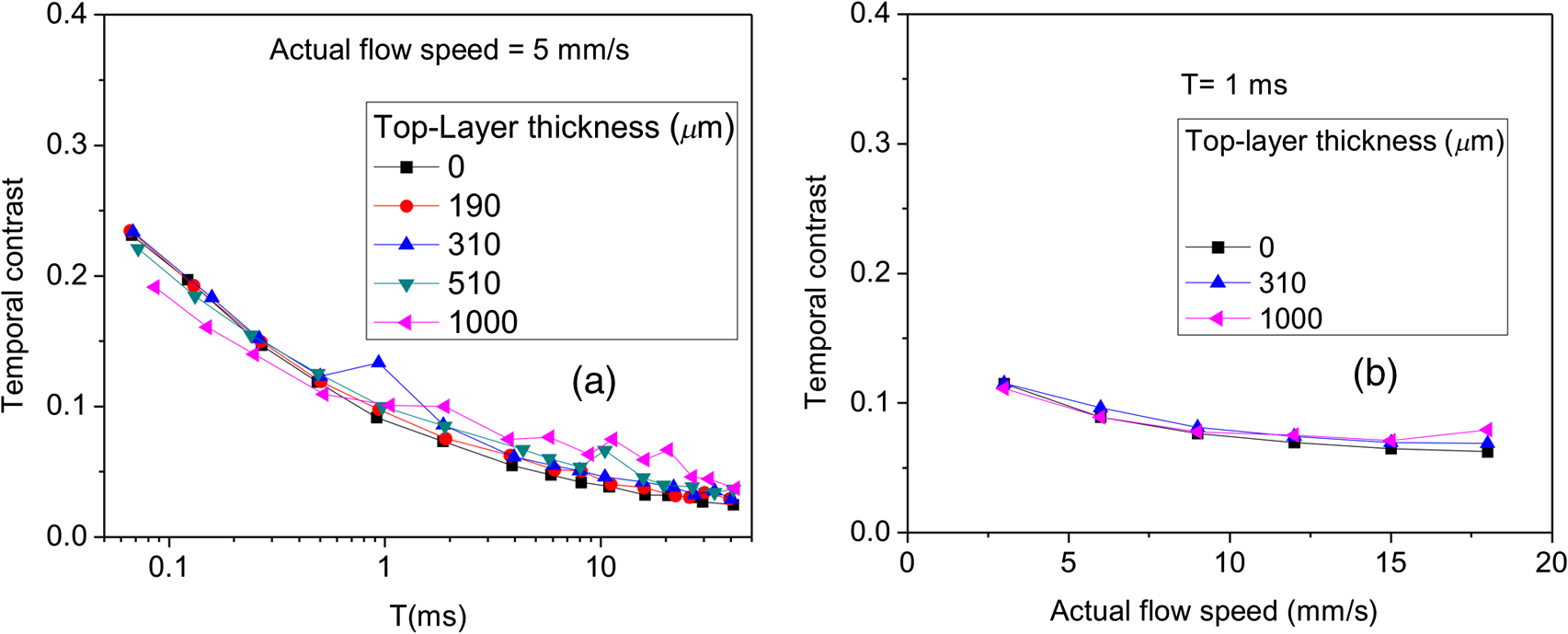
1.IntroductionLaser speckle contrast imaging (LSCI) is an optical technique based on calculating the contrast of an integrated speckle pattern, which allows us to analyze the dynamics of blood flow.1 LSCI has attracted attention because it is able to image blood flow in skin,2 retina,3 and brain4 at relatively high spatial and temporal resolutions and without the need for scanning of the region of interest. Additionally, it is simple and inexpensive relative to similar laser Doppler-based techniques.5,6 During the last decade, the theoretical model behind LSCI has evolved to include modifications to the original Fercher and Briers model,7 taking into account the effects of static optical scatterers,8,9 as well as the ratio of pixel and speckle sizes,10–13 resulting in the following speckle imaging equation: where is the local contrast of the raw speckle image at the pixel (); is a normalization parameter; is the area of the pixel divided by the diffraction-limited area of the minimally resolvable speckle; is the fraction of light reaching the pixel () that interacts with moving optical scatterers; and , where is the exposure time of the CCD camera and is the correlation time of the light intensity.Research groups proposed various approaches to calculate the speckle contrast from a raw speckle image or set of images.14 Spatial analysis,15 probably the most common approach, implements a sliding, square structuring element of or pixels to calculate the local speckle contrast as the standard deviation of pixel intensities () divided by the mean intensity () within the element boundaries. Ideally, the speckle area should be at least twice the pixel area10 to minimize detrimental effects because of spatial integration of the speckle pattern;11 otherwise, a correction factor should be applied to the measured speckle contrast.13 The spatial algorithm requires only one raw speckle image to compute a contrast image, and therefore offers high-temporal resolution at the expense of spatial resolution because of the use of the structuring element. To circumvent the reduction in spatial resolution, Cheng et al.16 proposed a temporal algorithm that calculates a speckle contrast image by computing for each pixel across a sequence of images. This approach requires a minimum of 15 statistically independent images16 and is associated with better spatial resolution at the expense of temporal resolution. Recent studies describe results that support the use of the temporal algorithm to analyze raw speckle images. We discovered that the temporal algorithm is more accurate than the spatial algorithm at assessing the relative change in flow speed.12 This improved accuracy appears to be from the reduction in sensitivity of temporal analysis to the presence of static optical scatterers.8,9,17 Li et al.18 reported that the temporal algorithm enabled visualization of subsurface () blood vessels through the intact rat skull; these vessels were not visible in spatial speckle contrast images. Here, we report on in vitro experiments that extend upon our understanding of temporal speckle contrast analysis. Specifically, we focused on the quantitation of speckle contrast and the impact of depth of fluid flow on speckle contrast values. We studied these effects using two clinically relevant imaging geometries: epi-illumination and transillumination. 2.Materials and MethodsWe used two separate phantom setups for the experiments described in this paper: (1) an epi-illuminated skin-simulating phantom (Fig. 1), and (2) a transilluminated excised human tooth (Fig. 2). Fig. 1Experimental setup used for epi-illumination experiments. We infused 5% Intralipid into a glass capillary tube embedded at different depths from the surface of a two-layer silicone phantom geometry. We used epi-illumination with an 808-nm laser and collected raw speckle images with a cooled CCD camera.  Fig. 2Experimental setup used for transillumination experiments. We infused Intralipid through Tygon tubing threaded through the tooth model. We transilluminated the tooth with a 632.8-nm laser and collected images with a CCD camera via a fiber bundle.  2.1.Skin-Simulating PhantomWe constructed the skin-simulating phantom using a silicone block containing appropriate concentrations of to mimic the reduced scattering coefficient () of biological tissue at visible and near-infrared wavelengths (Fig. 1). We embedded a glass capillary tube, with an inner diameter of , at the surface of the block. We placed a second thin silicone skin-simulating phantom of varying thicknesses (190 to ) on top of the block to mimic the overlying tissue. We fabricated the thin phantoms using powder and coffee to simulate the optical scattering and absorption coefficients, respectively, of the epidermis.19 By using different thicknesses of the overlying layer, we effectively modulated . For laser speckle imaging (LSI) with epi-illumination, we used an 808-nm laser (Ondax, Monrovia, California) as the excitation source, with a variable attenuator to adjust the intensity of illumination and ground-glass diffuser to expand and homogenize the incident laser light (spot illumination: 5-mm diameter). A Retiga EXi FAST cooled CCD camera (QImaging, Surrey, BC, Canada) collected the raw speckle images at 20 fps. The camera was equipped with a macrolens (Nikon, Melville, New York), with an aperture setting of . We acquired images using Q-Capture Pro v5.1 software and selected the exposure time using the autoexpose function. We collected images of the phantom at exposure times ranging between and 43 ms by using the variable attenuator to change the irradiance of the excitation light. We collected data from the phantom with the following configurations: no top layer present (i.e., microchannel at surface of phantom) and with overlying top-layer thicknesses (TLTs) of 190 m, 310, 510, and . We used a syringe pump (Harvard Apparatus, Holliston, Massachusetts) to infuse 5% Intralipid solution as a blood surrogate (Baxter Healthcare, Deerfield, Illinois) into the channel at speeds of 0 to . 2.2.Tooth-Simulating PhantomWe also simulated transillumination LSI conditions, recently proposed by Stoianovici et al.,20 for the study of pulpal blood flow in teeth (Fig. 2). Teeth are well suited for transillumination LSI because of the highly forward scattering feature of interior dentine tubules.21 We used an excised human adult molar as a phantom. We drilled a small hole from the middle of the occlusal surface of the tooth to the bottom of the tooth between the roots. We inserted a Tygon tube with an inner diameter of into the hole and connected it to a syringe pump. Our experimental setup consisted of a configuration currently under investigation for study of pulpal blood flow. We illuminated the tooth on one side with a fiber-coupled 632.8-nm HeNe laser (JDSU, Milpitas, California). On the opposite side of the tooth, we positioned a leached fiber bundle (Schott, Southbridge, Massachusetts)22 with a drum lens to focus the image on to a CCD camera (Flea3, Point Gray, Richmond, BC, Canada). We acquired images with FlyCap software (Point Gray) at a fixed exposure time of 10 ms and a gain of 24 dB. For this experiment, we calculated spatial and temporal contrasts in two regions of interest, one on the left side of the tooth and the other on the right. The tooth was approximately thicker on the right side than the left, effectively resulting in different at the two interrogated regions. With both experimental setups, we collected a sequence of 30 images per experimental condition and processed with both spatial and temporal speckle imaging algorithms. With the spatial algorithm, we used a sliding pixel structuring element to calculate maps of speckle contrast from each acquired raw speckle image and obtained a final contrast image by averaging the 30 contrast images.15 We calculated temporal contrast on a pixel-by-pixel basis, across all 30 images in the sequence.16 All values shown in the data figures (Figs. 3Fig. 4Fig. 5–6) represent the average contrast in a region of interest () positioned over the center of the tube. Fig. 3(a) Spatial speckle contrast increased with increasing top-layer thickness (TLT) at a given exposure time (). The symbols represent the experimental data and the continuous lines data fits using Eq. (1). (b) At , for a given actual flow speed value, spatial speckle contrast increased with increasing TLT. 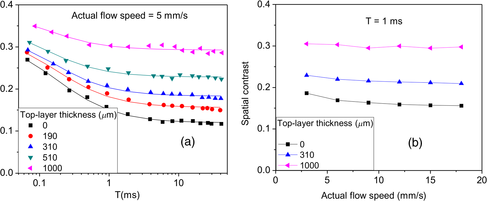 Fig. 4Spatial speckle contrast depends strongly on the fraction of nonmoving optical scatterers (e.g., ) and hence on the TLT. (a) decreases in exponential fashion with TLT, and increases in linear fashion with TLT. Solid points represent the experimental data, and lines represent the fits to the data. (b) The sensitivity of to exposure time depends strongly on TLT, for short (), the sensitivity decreases for thicker TL and for , the expected value of the contrast is constant [see Fig. 3(a)] and therefore the sensitivity approaches to zero.  3.Results and Discussion3.1.Skin-Simulating PhantomSimilar to previously published data,8 for a given TLT, we observed that the spatial speckle contrast decreased with an increase in [Fig. 3(a)]. For a given , with an increase in TLT, the contrast increased because of a decrease in . For a given flow speed, the contrast increased with an increase in TLT [Fig. 3(b)]. Collectively, these data demonstrate that, for flow in a subsurface tube, the spatial speckle contrast analysis is incapable of enabling unambiguous assessment of flow speed within the tube. For a given TLT [Fig. (3a)], the spatial speckle contrast was maximum () at the shortest , and then asymptotically decayed to a minimum (). For a given , the dynamic range of spatial speckle contrast (i.e., ) decreased with increasing TLT, because of a corresponding decrease in . We fit Eq. (1) to the experimental data in Fig. 3(a) to estimate , , and . From the fitting results, the mean value of was , which is similar to the values reported by Parthasarathy et al.8 for similar flow speed. and are plotted versus TLT in Fig. 4. For a given actual flow speed, we observe an exponential decay of with an increase in TLT [Fig. 4(a)], which we postulate is associated with the exponential behavior of light attenuation described by Beer’s law. Because of the asymptotic behavior of with increasing (and hence increasing ), we determine as where [0,1]. From Eq. (2), we see that decreases in a linear fashion with a decrease in TLT [Fig. 4(a)]. From the first derivative of Eq. (1), we see that the sensitivity of spatial speckle contrast () decreases with an increase in TLT [Fig. 4(b)]. Collectively, our experimental data and analysis using Eq. (1) demonstrate that the spatial speckle contrast has a strong dependence on the fraction of nonmoving optical scatterers (e.g., ), which in turn depends on the TLT. Hence, spatial speckle contrast analysis is incapable of accurate quantitation of subsurface flow dynamics because of the impact of TLT on .Previous reports8,12,18 present data that strongly suggest that the temporal speckle contrast is altered primarily by temporal variations in light remitted from the sample and considerably less sensitive to static optical scatterers. We set out to determine the degree to which temporal contrast depends on specific independent variables. We find that the temporal contrast decreases with increasing [Fig. 5(a)] and increasing flow speed [Fig. 5(b)], but we also observed that the contrast is relatively independent of TLT for a wide range of values (0 to ; Fig. 5). 3.2.Tooth-Simulating PhantomWe also studied this relationship using a transillumination LSI configuration, a setup previously proposed for study of teeth20 and joints,23 and used routinely by our group to assess the blood flow in the rodent dorsal window chamber model.24 We used a tooth model in which the thickness of the right side of the tooth was approximately thicker than the left side, resulting in a higher proportion of static scatterers (i.e., lower ). Similar to the data collected with the epi-illumination setup, we observed that the spatial contrast depends on TLT [Fig. 6(a)], and temporal contrast is independent of TLT [Fig. 6(b)]. In this work, we studied the impact of overlying optical scatterers on measurements of speckle contrast. We used two different imaging setups and both spatial and temporal contrast analyses. With spatial analysis and epi-illumination, we determined that the speckle contrast offset increases in a linear fashion with TLT [Fig. 4(a)] and the sensitivity of speckle contrast decreased with an increase in TLT [Fig. 4(b)]. With temporal speckle contrast analysis (Fig. 5), speckle contrast measurements were remarkably independent of TLT, presumably due to the relative immunity of temporal contrast to contributions from static optical scatterers.16–18 Our data demonstrate that the temporal contrast analysis can characterize accurately speckle contrast because of subsurface moving scatterers for TLT as thick as 1 mm, and for a wide range of and flow speeds. We observed similar results with a transillumination geometry. Collectively, these results strongly suggest the potential of temporal LSI at a single-exposure time to assess the changes in blood flow even in the presence of substantial static optical scattering, which can ultimately be combined with methods to improve the localization of speckle contrast such as spatial frequency domain25,26 or magnetomotive techniques.27 AcknowledgmentsThis research was funded in part by CONACYT (CB-2010-156876-F), the Arnold and Mabel Beckman Foundation, and the National Institutes of Health (P41 EB015890, R01 DE022831, and R01 HD065536). ReferencesA. F. FercherJ. D. Briers,
“Flow visualization by means of single-exposure speckle photography,”
Opt. Commun., 37
(5), 326
–330
(1981). http://dx.doi.org/10.1016/0030-4018(81)90428-4 OPCOB8 0030-4018 Google Scholar
B. ChoiN. M. KangJ. S. Nelson,
“Laser speckle imaging for monitoring blood flow dynamics in the in vivo rodent dorsal skin fold model,”
Microvasc. Res., 68
(2), 143
–146
(2004). http://dx.doi.org/10.1016/j.mvr.2004.04.003 MIVRA6 0026-2862 Google Scholar
Y. Tamakiet al.,
“Noncontact, two-dimensional measurement of tissue circulation in choroid and optic nerve head using laser speckle phenomenon,”
Exp. Eye Res., 60
(4), 373
–383
(1995). http://dx.doi.org/10.1016/S0014-4835(05)80094-6 EXERA6 0014-4835 Google Scholar
A. K. Dunnet al.,
“Dynamic imaging of cerebral blood flow using laser speckle,”
J. Cereb. Blood Flow Metab., 21 195
–201
(2001). http://dx.doi.org/10.1097/00004647-200103000-00002 JCBMDN 0271-678X Google Scholar
K. Yaoedaet al.,
“Measurement of microcirculation in the optic nerve head by laser speckle flowgraphy and scanning laser Doppler flowmetry,”
Am. J. Ophthalmol., 129
(6), 734
–739
(2000). http://dx.doi.org/10.1016/S0002-9394(00)00382-2 AJOPAA 0002-9394 Google Scholar
C. RivaB. RossG. B. Benedek,
“Laser Doppler measurements of blood flow in capillary tubes and retinal arteries,”
Invest. Ophthalmol., 11
(11), 936
–944
(1972). INOPAO 0020-9988 Google Scholar
R. Bandyopadhyayet al.,
“Speckle-visibility spectroscopy: a tool to study time-varying dynamics,”
Rev. Sci. Instrum., 76 093110
(2005). http://dx.doi.org/10.1063/1.2037987 RSINAK 0034-6748 Google Scholar
A. B. Parthasarathyet al.,
“Robust flow measurement with multi-exposure speckle imaging,”
Opt. Express, 16
(3), 1975
–1989
(2008). http://dx.doi.org/10.1364/OE.16.001975 OPEXFF 1094-4087 Google Scholar
D. A. BoasA. K. Dunn,
“Laser speckle contrast imaging in biomedical optics,”
J. Biomed. Opt., 15
(1), 011109
(2010). http://dx.doi.org/10.1117/1.3285504 JBOPFO 1083-3668 Google Scholar
S. J. KirkpatrickD. D. DuncanE. M. Wells-Gray,
“Detrimental effects of speckle-pixel size matching in laser speckle contrast imaging,”
Opt. Lett., 33
(24), 2886
–2888
(2008). http://dx.doi.org/10.1364/OL.33.002886 OPLEDP 0146-9592 Google Scholar
O. ThompsonM. AndrewsE. Hirst,
“Correction for spatial averaging in laser speckle contrast analysis,”
Biomed. Opt. Express, 2
(4), 1021
–1029
(2011). http://dx.doi.org/10.1364/BOE.2.001021 BOEICL 2156-7085 Google Scholar
J. C. Ramirez-San-Juanet al.,
“Effects of speckle/pixel size ratio on temporal and spatial speckle-contrast analysis of dynamic scattering systems: implication for measurements of blood-flow dynamics,”
Biomed. Opt. Express, 4
(10), 1883
–1889
(2013). http://dx.doi.org/10.1364/BOE.4.001883 BOEICL 2156-7085 Google Scholar
J. C. Ramirez-San-Juanet al.,
“Simple correction factor for laser speckle imaging of flow dynamics,”
Opt. Lett., 39
(3), 678
–681
(2014). http://dx.doi.org/10.1364/OL.39.000678 OPLEDP 0146-9592 Google Scholar
M. Draijeret al.,
“Review of laser speckle contrast techniques for visualizing tissue perfusion,”
Lasers Med. Sci., 24
(4), 639
–651
(2009). http://dx.doi.org/10.1007/s10103-008-0626-3 LMSCEZ 1435-604X Google Scholar
J. D. BriersS. Webster,
“Quasi real-time digital version of single-exposure speckle photography for full-field monitoring of velocity or flow fields,”
Opt. Commun., 116
(1–3), 36
–42
(1995). http://dx.doi.org/10.1016/0030-4018(95)00042-7 OPCOB8 0030-4018 Google Scholar
H. Chenget al.,
“Modified laser speckle imaging method with improved spatial resolution,”
J. Biomed. Opt., 8
(3), 559
–564
(2003). http://dx.doi.org/10.1117/1.1578089 JBOPFO 1083-3668 Google Scholar
H. ChengY. YanT. Q. Duong,
“Temporal statistical analysis of laser speckle images and its application to retinal blood-flow imaging,”
Opt. Express, 16
(14), 10214
–10219
(2008). http://dx.doi.org/10.1364/OE.16.010214 OPEXFF 1094-4087 Google Scholar
P. Liet al.,
“Imaging cerebral blood flow through the intact rat skull with temporal laser speckle imaging,”
Opt. Lett., 31
(12), 1824
–1826
(2006). http://dx.doi.org/10.1364/OL.31.001824 OPLEDP 0146-9592 Google Scholar
R. B. Saageret al.,
“Multi-layer silicone phantoms for the evaluation of quantitative optical techniques in skin imaging,”
Proc. SPIE, 7567 756706
(2010). http://dx.doi.org/10.1117/12.842249 PSISDG 0277-786X Google Scholar
C. StoianoviciP. Wilder-SmithB. Choi,
“Assessment of pulpal vitality using laser speckle imaging,”
Lasers Surg. Med., 43
(8), 833
–837
(2011). http://dx.doi.org/10.1002/lsm.21090 LSMEDI 0196-8092 Google Scholar
S. KakinoY. TakagiS. Takatani,
“Absolute transmitted light plethysmography for assessment of dental pulp vitality through quantification of pulp chamber hematocrit by a three-layer model,”
J. Biomed. Opt., 13
(5), 054023
(2008). http://dx.doi.org/10.1117/1.2976112 JBOPFO 1083-3668 Google Scholar
S. K. Nadkarniet al.,
“Laser speckle imaging of atherosclerotic plaques through optical fiber bundles,”
J. Biomed. Opt., 13
(5), 054016
(2008). http://dx.doi.org/10.1117/1.2982529 JBOPFO 1083-3668 Google Scholar
J. F. Dunnet al.,
“A transmissive laser speckle imaging technique for measuring deep tissue blood flow: an example application in finger joints,”
Lasers Surg. Med., 43
(1), 21
–28
(2011). http://dx.doi.org/10.1002/lsm.v43.1 LSMEDI 0196-8092 Google Scholar
A. J. Moyet al.,
“Wide-field functional imaging of blood flow and hemoglobin oxygen saturation in the rodent dorsal window chamber,”
Microvasc. Res., 82
(3), 199
–209
(2011). http://dx.doi.org/10.1016/j.mvr.2011.07.004 MIVRA6 0026-2862 Google Scholar
A. Mazharet al.,
“Wavelength optimization for rapid chromophore mapping using spatial frequency domain imaging,”
J. Biomed. Opt., 15
(6), 061716
(2010). http://dx.doi.org/10.1117/1.3523373 JBOPFO 1083-3668 Google Scholar
T. B. Riceet al.,
“Quantitative, depth-resolved determination of particle motion using multi-exposure, spatial frequency domain laser speckle imaging,”
Biomed. Opt. Express, 4
(12), 2880
–2892
(2013). http://dx.doi.org/10.1364/BOE.4.002880 BOEICL 2156-7085 Google Scholar
J. KimJ. OhB. Choi,
“Magnetomotive laser speckle imaging,”
J. Biomed. Opt., 15
(1), 011110
(2010). http://dx.doi.org/10.1117/1.3285612 JBOPFO 1083-3668 Google Scholar
|