1.

Introduction

Key tissue parameters, e.g., total hemoglobin concentration and tissue oxygenation, are important biomarkers in clinical diagnosis for various diseases.¹ The previous studies have shown that diffuse reflectance spectroscopy can be used to accurately recover these parameters noninvasively using different methods, such as Monte Carlo-based inverse model,² diffusion theory-based model,³ and the look-up table method.⁴ However, the common disadvantage of traditional diffuse reflectance spectroscopy is slow data acquisition when multiple locations need to be measured.⁵ This is attributed to the employment of fiber-optic probes in traditional diffuse reflectance spectroscopy, which can only perform point measurements. Slow data acquisition prohibits the use of diffuse reflectance spectroscopy in those applications in which the observation of fast changing phenomena is required.

Several spectral imaging techniques are developed to speed up the data acquisition. Multispectral imaging^6–8 captures image data at certain wavelengths using specific filters or instruments that are sensitive to particular wavelengths instead of the entire spectrum. The advantage of this technique is that both the spectral and spatial information can be recorded simultaneously.⁹ However, the data acquisition is time consuming when high spectral resolution is required. This limitation originates from the employment of a wavelength selection/dispersion device in most imaging setups, for which information at only one or a couple of wavelengths can be collected in one measurement. Snapshot hyperspectral imaging is a technique in which both the spatial and spectral information are acquired simultaneously in a snap shot¹⁰ but in a coded manner. The key idea in snapshot hyperspectral imaging is that hyperspectral images can be captured all at once on a two-dimensional detector array. The disadvantage of snapshot hyperspectral imaging techniques is that data postprocessing is slow when the required spectral resolution is high. In addition, a large detector array is needed to properly sample a sufficient number of voxels and those large detector arrays are usually expensive. To overcome this limitation, spectral imaging can be realized by spectral reconstruction from wide-band measurements such as color imaging measurements, in which a method capable of fast and accurate spectral reconstruction is critical. Various methods have been explored to reconstruct diffuse reflectance spectra from wide-band measurements, which includes pseudo-inverse,¹¹ finite-dimensional modeling,¹² and Wiener estimation (WE).¹³ Our previous study⁵ has shown that diffuse reflectance spectra can be accurately recovered from in vivo color measurements on human skin. Therefore, it may be possible to directly derive tissue parameters from wide-band measurements.

Multiple early studies^14,15 have shown that hemoglobin concentration and oxygenation in tissue phantoms with known scattering properties can be estimated from color measurements in R(Red), G(Green), B(Blue) channels using a method involving Monte Carlo modeling and multiple steps of regression analysis. However, the scattering properties of tissues carry important physiological information,¹⁶ which are typically unknown and can vary significantly from one subject to another. To our best knowledge, there is no previous study in which both absorption and scattering properties are directly estimated from wide-band measurements in a tissue model with varying or unknown scattering properties.

In this study, we reported a method of sequential weighted WE to directly extract total hemoglobin concentration (${\mathrm{C}}_{\mathrm{tHb}}$), hemoglobin oxygenation (${\mathrm{StO}}_2$), scatterer density ($\alpha$), and scattering power ($\beta$) from wide-band measurements. This method takes advantage of the fact that each parameter is sensitive to the color measurements to a different degree and attempts to maximize the contribution of those color measurements that are more likely to generate correct results in the process of WE. The method was evaluated on tissue phantoms with varying ${\mathrm{C}}_{\mathrm{tHb}}$, ${\mathrm{StO}}_2$, and scattering properties to mimic human skin, in which a 3-charge coupled device (CCD) camera was used to capture the wide-band color measurements from the tissue phantoms. The results demonstrate excellent agreement between the estimated tissue parameters and the corresponding reference values. Compared with the traditional WE, the method of sequential weighted WE shows significant improvement, especially for hemoglobin oxygenation estimation. This method possesses great potential in the noninvasive and real-time monitoring of tissue parameters in an imaging setup to investigate fast changing phenomena.

2.

Materials and Methods

In this study, tissue phantoms with varying absorption, scattering, and oxygenation were used to mimic the human skin. Both traditional WE and sequential weighted WE were tested to extract tissue parameters, including the total hemoglobin concentration (${\mathrm{C}}_{\mathrm{tHb}}$), hemoglobin oxygenation (${\mathrm{StO}}_2$), scatterer density ($\alpha$), and scattering power ($\beta$). The leave-one-out method was used for cross validation and the genetic algorithm was utilized to find the optimal combination of coefficients. All the postprocessing steps, including the traditional WE, sequential weighted WE, leave-one-out method, and genetic algorithm, were coded and run in Matlab (R2011b, MathWorks, Natick, Massachusetts). The details in each step are described as follows.

2.1.

System Information

In this study, all the data were measured by the system shown in Fig. 1, which consisted of a white light source (UHP-Mic-LED-White, Prizmatix, Givat-Shmuel, Illinois), a 3-CCD (AT-200 GE, JAI, San Jose, California), a magnetic stirrer (97042-596, VWR, Radnor, Pennsylvania), and two linear polarizers (LPVISE100-A, Thorlabs, Newton, New Jersey). White light passed through the first linear polarizer, which was aligned such that its direction of polarization was parallel to the source-sample-detector plane. The illumination light was delivered at a fixed angle of 45 deg onto a sample to avoid the collection of specular reflectance.¹⁷ The second linear polarizer was put in front of the 3-CCD in order to acquire signals with two different polarization directions (parallel or perpendicular to the incident polarization). The signal detected with parallel polarization contained contributions from both the superficial and deep regions inside the phantom, in which photons responsible for contribution from the superficial are mostly scattered only a single or a few times.^18,19 Therefore, the signal detected with parallel polarization was expected to be sensitive to the scattering properties of the phantoms thus, in turn, to the scatterer density ($\alpha$) and scattering power ($\beta$). By contrast, the signal detected with perpendicular polarization contained only light from deep regions inside the phantom, which was expected to be sensitive to the absorption properties of the phantoms due to the long optical path length and to total hemoglobin concentration (${\mathrm{C}}_{\mathrm{tHb}}$) and hemoglobin oxygenation (${\mathrm{StO}}_2$). The sample was viewed by the camera right above, along the normal axis of the sample surface. A computer was connected to the camera to acquire the images of the sample, which contained the wide-band color measurements. Among these tissue parameters, hemoglobin concentration and oxygen saturation together determine the absorption coefficient spectrum according to Beer’s law, whereas the scattering amplitude and scattering power together determine the reduced scattering coefficient ${\mu }_{\mathrm{s}}^{\prime }$ for the whole visible spectrum ($\lambda$) by the following empirical equation:^20,21

Eq. (1)

$${\mu }_{\mathrm{s}}^{\prime }(\lambda )=\alpha {\lambda }^{-\beta }.$$

Fig. 1

Schematic of the color imaging system with devices measuring pH and dissolved oxygen in the sample. The red lines with arrows represent light flow.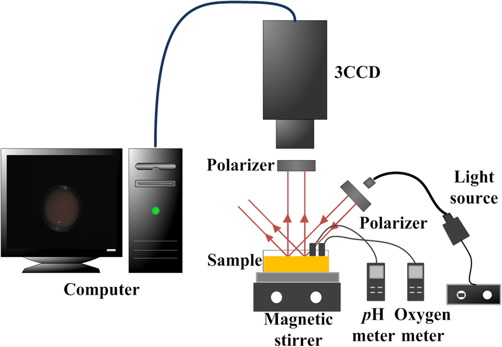

The spectra of absorption and scattering coefficients together with the configuration of optical measurements determine the diffuse reflectance spectrum. After passing through the RGB (i.e., Red, Green, and Blue) filters, the diffuse reflectance spectrum is transformed to RGB values, as shown in Eq. (2):

Eq. (2)

$$C=FS,$$

where $C$ is the RGB responses, $F$ represents the transmission spectra of RGB filters, and $S$ is the diffuse reflectance spectrum. Therefore, the RGB responses and their ratios are determined by these tissue parameters and, therefore, contain the information of all the tissue parameters. A pH meter and thermometer (HI 9024, Sigma-Aldrich, St. Louis, Missouri) and a dissolved oxygen meter (HI 9142, Sigma-Aldrich, St. Louis, Missouri) were used to measure the pH value, temperature, and oxygen level in the phantom sample, respectively, which were used to derive hemoglobin oxygenation. The relative emission spectrum of the white light source, the relative spectral response of the 3-CCD, and the transmittance of the polarizers are shown in Fig. 2.

Fig. 2

(a) Relative emission spectrum of white light source, (b) relative spectral response of the 3-CCD, and (c) transmittance of the polarizer.

2.3.

Data Analysis

2.3.1.

Sequential weighted WE

In traditional WE, when ignoring the noise term, the Wiener matrix is formulated as

Eq. (3)

$$W=E[s{c}^{\mathrm{T}}]{[E[c{c}^{\mathrm{T}}]]}^{-1},$$

where the superscript “T” represents the matrix transpose, the superscript “$-1$” represents the matrix inverse, $E[]$ represents the ensemble average, $s$ represents the tissue parameters, and $c$ represents the wide-band measurements. More details for traditional WE have been reported elsewhere.³¹ In the weighted WE that we developed, the ensemble average is replaced by the weighted average as shown in Eq. (4):

Eq. (4)

$$W=\sum _{i=1}^n{w}_i{s}_i{c}_i^T\sum _{j=1}^n{(w_j{c}_j{c}_j^T)}^{-1},$$

where $w_i$ or $w_j$ is the weight for the $i$’th or $j$’th set of calibration data. This weight is calculated according to the following equation:

Eq. (5)

$$w_i=\frac{D_i^m}{\sum _{i=1}^n{D}_i^m},$$

where $D_i$ is the similarity between the tissue parameter value estimated from the test data and the corresponding parameter value in the $i$’th set of tissue parameters in the calibration data and $m$ is the power to adjust the contribution of $D_i$. The similarity $D_i$ is calculated according to Eq. (6):

Eq. (6)

$$D_i=\frac{d_i^{-1}}{\sum _{i=1}^n{d}_i^{-1}},$$

where $d_i$ denotes the difference between the tissue parameter value estimated from the test data and the corresponding parameter value in the $i$’th set of tissue parameters in the calibration data and $m$ is the power to adjust the contribution of $d_i$. When multiple estimated tissue parameters need to be included in the weighting scheme, the corresponding similarity values will be calculated separately according to Eq. (6) and then averaged to yield a single similarity value. The accuracy of the estimation can be improved by using a large number of calibration data highly similar to the test data set. According to Eqs. (5) and (6), any calibration data with a set of tissue parameter values very different from the test data would yield a tiny weight, which makes a nearly negligible contribution to the weighted Wiener matrix by Eq. (4). According to the same equations, a larger $m$ generates a more effective calibration data set, which is more similar to the test data set, than a smaller $m$ does. However, if $m$ becomes too large, the weight can be very small not only for those calibration data very different from the test data but also for those calibration data moderately similar to the test data by Eqs. (5) and (6). As a result, the effective calibration data will be much less because only those very similar to the test data are retained. Such a small set of calibration data is likely to yield large errors in estimation when the calibration data or the test data contain measurement uncertainty or noises. Therefore, the adjustment of $m$ is the tradeoff between the population size of the effective calibration data and the similarity between the calibration data set and the test data set, when the full calibration data set is fixed. The value of $m$ was fixed at 5 in this study to achieve the tradeoff. According to Eq. (4) to Eq. (6), the summation of $w_i$ is 1, and the contribution of a set of calibration data to the Wiener matrix is proportional to the similarity between the estimated tissue parameters in the test data set and the $i$’th set of tissue parameters in the calibration data.

The schematic of the sequential weighted WE is shown in Fig. 3. This method consists of multiple steps of estimation that can be run iteratively, in which the parameters in the order of estimation are the scattering power ($\beta$), the total hemoglobin concentration (${\mathrm{C}}_{\mathrm{tHb}}$), the scatterer density ($\alpha$), and hemoglobin oxygenation (${\mathrm{StO}}_2$). The estimation error of each individual parameter when using traditional WE decreases with this order in the calibration stage; therefore, this order will prevent the early estimation error from propagating to the later estimation. In the first step, the scattering power $\beta$ is extracted using a traditional WE method. Then, ${\mathrm{C}}_{\mathrm{tHb}}$ is estimated using the weighted WE as in Eq. (4) and the weights are calculated using Eqs. (5) and (6) according to the difference between the $\beta$ value estimated from the test data and the $\beta$ values in the calibration data. After that, $\alpha$ is estimated using the weighted WE as in Eq. (4) and the weights are calculated using Eqs. (5) and (6) according to the difference between ${\mathrm{C}}_{\mathrm{tHb}}$ and $\beta$ values estimated from the test data and these values in the calibration data. Finally, ${\mathrm{StO}}_2$ is estimated using the weighted WE as in Eq. (4) and the weights are calculated according to the difference between ${\mathrm{C}}_{\mathrm{tHb}}$, $\alpha$, and $\beta$ values estimated from the test data and these values in the calibration data. This completes one loop in the sequential weighted WE. If the estimated results are not satisfactory, the loop can be run again, in which $\beta$ will be calculated again according to the weights calculated according to the similarity between ${\mathrm{C}}_{\mathrm{tHb}}$, ${\mathrm{StO}}_2$ and $\alpha$ values estimated from the test data in the first loop and those values in the calibration data. All the steps can be repeated iteratively until the estimated results are acceptable.

Fig. 3

Schematic of sequential weighted Wiener estimation (WE).

2.3.2.

Leave-one-out method, genetic algorithm and evaluation criterion

The leave-one-out method³² was used for cross validation. In this strategy, data measured from one tissue phantom are used for testing and data measured from other tissue phantoms are used for calibration. Then a new tissue phantom is selected for testing and the procedure is repeated until all the tissue phantoms have been tested.

Because the ratios of wide-band measurements contained important information about hemoglobin,^33,34 we examined both the absolute values of wide-band measurements and their ratios. These two sets of data were named jointly as coefficients in Table 1. A genetic algorithm was used to find the optimal combination of the coefficients for the estimation of each tissue parameter. The optimization methodology proceeded in the following manner. First, a population of coefficient combination was initialized randomly. Second, the traditional WE (for comparison) or sequential weighted WE was applied to extract the tissue parameters and the accuracy of the recovered tissue parameters was evaluated. The accuracy was quantified according to the relative root mean square error (RMSE) calculated from Eq. (7). Third, a new population of coefficient combination was generated according to the accuracy of the recovered tissue parameters, in which the coefficient combination yielding a higher accuracy was more likely to become the parent of the new population. The crossover rate was 0.9 and the mutation rate was 0.1. The second and third steps were repeated iteratively until an optimized combination of coefficient was found:

Eq. (7)

$$\text{Relative}\mathrm{RMSE}=\sqrt{\frac{\sum _{i=1}^n{\left(\frac{i\prime \mathrm{th}\text{estimated}\text{parameter}-i\prime \mathrm{th}\text{reference}\text{parameter}}{i\prime \mathrm{th}\text{reference}\text{parameter}}\right)}^2}{n}}.$$

Table 1

Coefficients for estimation of tissue parameters.a

Indices	Coefficients
$1\sim 12$	${\mathrm{R}}_{\parallel }$, ${\mathrm{G}}_{\parallel }$, ${\mathrm{B}}_{\parallel }$, ${\mathrm{R}}_{\perp }$, ${\mathrm{G}}_{\perp }$, ${\mathrm{B}}_{\perp }$, ${\mathrm{R}}_{\text{sum}}$, ${\mathrm{G}}_{\text{sum}}$, ${\mathrm{B}}_{\text{sum}}$, ${\mathrm{R}}_{\mathrm{sub}}$, ${\mathrm{G}}_{\mathrm{sub}}$, ${\mathrm{B}}_{\mathrm{sub}}$
$13\sim 24$	${\mathrm{R}}_{\parallel }/({\mathrm{R}}_{\parallel }+{\mathrm{G}}_{\parallel }+{\mathrm{B}}_{\parallel })$, ${\mathrm{G}}_{\parallel }/({\mathrm{R}}_{\parallel }+{\mathrm{G}}_{\parallel }+{\mathrm{B}}_{\parallel })$, ${\mathrm{B}}_{\parallel }/({\mathrm{R}}_{\parallel }+{\mathrm{G}}_{\parallel }+{\mathrm{B}}_{\parallel })$, ${\mathrm{R}}_{\perp }/({\mathrm{R}}_{\perp }+{\mathrm{G}}_{\perp }+{\mathrm{B}}_{\perp })$, ${\mathrm{G}}_{\perp }/({\mathrm{R}}_{\perp }+{\mathrm{G}}_{\perp }+{\mathrm{B}}_{\perp })$, ${\mathrm{B}}_{\perp }/({\mathrm{R}}_{\perp }+{\mathrm{G}}_{\perp }+{\mathrm{B}}_{\perp })$, ${\mathrm{R}}_{\text{sum}}/({\mathrm{R}}_{\text{sum}}+{\mathrm{G}}_{\text{sum}}+{\mathrm{B}}_{\text{sum}})$, ${\mathrm{G}}_{\text{sum}}/({\mathrm{R}}_{\text{sum}}+{\mathrm{G}}_{\text{sum}}+{\mathrm{B}}_{\text{sum}})$, ${\mathrm{B}}_{\text{sum}}/({\mathrm{R}}_{\text{sum}}+{\mathrm{G}}_{\text{sum}}+{\mathrm{B}}_{\text{sum}})$, ${\mathrm{R}}_{\mathrm{sub}}/({\mathrm{R}}_{\mathrm{sub}}+{\mathrm{G}}_{\mathrm{sub}}+{\mathrm{B}}_{\mathrm{sub}})$, ${\mathrm{G}}_{\mathrm{sub}}/({\mathrm{R}}_{\mathrm{sub}}+{\mathrm{G}}_{\mathrm{sub}}+{\mathrm{B}}_{\mathrm{sub}})$, ${\mathrm{B}}_{\mathrm{sub}}/({\mathrm{R}}_{\mathrm{sub}}+{\mathrm{G}}_{\mathrm{sub}}+{\mathrm{B}}_{\mathrm{sub}})$
$25\sim 36$	${\mathrm{R}}_{\parallel }/{\mathrm{G}}_{\parallel }$, ${\mathrm{R}}_{\parallel }/{\mathrm{B}}_{\parallel }$, ${\mathrm{G}}_{\parallel }/{\mathrm{R}}_{\parallel }$, ${\mathrm{G}}_{\parallel }/{\mathrm{B}}_{\parallel }$, ${\mathrm{B}}_{\parallel }/{\mathrm{R}}_{\parallel }$, ${\mathrm{B}}_{\parallel }/{\mathrm{G}}_{\parallel }$, ${\mathrm{R}}_{\perp }/{\mathrm{G}}_{\perp }$, ${\mathrm{R}}_{\perp }/{\mathrm{B}}_{\perp }$, ${\mathrm{G}}_{\perp }/{\mathrm{R}}_{\perp }$, ${\mathrm{G}}_{\perp }/{\mathrm{B}}_{\perp }$, ${\mathrm{B}}_{\perp }/{\mathrm{R}}_{\perp }$, ${\mathrm{B}}_{\perp }/{\mathrm{G}}_{\perp }$
$37\sim 48$	${\mathrm{R}}_{\text{sum}}/{\mathrm{G}}_{\text{sum}}$, ${\mathrm{R}}_{\text{sum}}/{\mathrm{B}}_{\text{sum}}$, ${\mathrm{G}}_{\text{sum}}/{\mathrm{R}}_{\text{sum}}$, ${\mathrm{G}}_{\text{sum}}/{\mathrm{B}}_{\text{sum}}$, ${\mathrm{B}}_{\text{sum}}/{\mathrm{R}}_{\text{sum}}$, ${\mathrm{B}}_{\text{sum}}/{\mathrm{G}}_{\text{sum}}$, ${\mathrm{R}}_{\mathrm{sub}}/{\mathrm{G}}_{\mathrm{sub}}$, ${\mathrm{R}}_{\mathrm{sub}}/{\mathrm{B}}_{\mathrm{sub}}$, ${\mathrm{G}}_{\mathrm{sub}}/{\mathrm{R}}_{\mathrm{sub}}$, ${\mathrm{G}}_{\mathrm{sub}}/{\mathrm{B}}_{\mathrm{sub}}$, ${\mathrm{B}}_{\mathrm{sub}}/{\mathrm{R}}_{\mathrm{sub}}$, ${\mathrm{B}}_{\mathrm{sub}}/{\mathrm{G}}_{\mathrm{sub}}$

^aR, red value; G, green value; B, blue value; ∥, light with parallel polarization; ⊥, light with perpendicular polarization; sum, ∥ + ⊥; sub, ∥ − ⊥.

3.

Results

Table 2 shows the relative RMSEs in the parameters estimated using traditional WE and the sequential weighted WE relative to the reference values. Out of four parameters estimated, i.e., ${\mathrm{C}}_{\mathrm{tHb}}$, ${\mathrm{StO}}_2$, scatterer density $\alpha$, and scattering power $\beta$, the relative RMSEs increase from the lowest to the highest for traditional WE in the order of $\beta$, ${\mathrm{C}}_{\mathrm{tHb}}$, $\alpha$, and ${\mathrm{StO}}_2$, and the sequential weighted WE performs estimations in the same sequence as shown in Fig. 3. The first weighted WE denotes the sequential weighted WE with only one iteration and the second weighted WE denotes the sequential weighted WE with two iterations. The relative RMSEs in estimated tissue parameters after the first-iteration weighted WE are 71.0%, 22.2%, 19.9% and 92.7% of those after traditional WE for ${\mathrm{C}}_{\mathrm{tHb}}$, ${\mathrm{StO}}_2$, $\alpha$, and $\beta$, respectively. The relative RMSEs after the second-iteration weighted WE are 24.1%, 96.5%, 94.4% and 49.3% of those after the first weighted WE for the same parameters. The decreases in the relative RMSEs of parameters indicate that the sequential weighted WE improves the estimation as the number of iteration increases.

Table 2

Relative RMSEs in the parameters estimated using traditional WE and sequential weighted WE relative to the reference values.

Figure 4 graphically shows the comparison between estimated parameters and reference parameters in the traditional WE and sequential weighted WE. It is observed that the markers representing the weighted WE stay much more packed and closer to the ideal lines than those representing the traditional WE, which suggests that the weighted WE, especially after two iterations, is more effective in the quantification of these parameters.

Fig. 4

(a) Total hemoglobin concentration ${\mathrm{C}}_{\mathrm{tHb}}$, (b) hemoglobin oxygenation ${\mathrm{StO}}_2$, (c) scatterer density $\alpha$, and (d) scattering power $\beta$ estimated using the traditional WE and weighted WE as a function of the expected value. The legend “1st weighted” means the result after the first iteration of weighted WE and the legend “2nd weighted” means the result after the second iteration of weighted WE.

The best combination of coefficients for estimating ${\mathrm{C}}_{\mathrm{tHb}}$, ${\mathrm{StO}}_2$, $\alpha$, and $\beta$ in the traditional WE, the first-iteration weighted WE, and the second-iteration weighted WE are shown in Table 3. It is interesting to observe that not only the best combination but also the number of coefficients in the best combination change from the traditional WE to the weighted WE as well as from the first iteration to the second iteration in the weighted WE.

Table 3

The best combination of coefficients for estimating CtHb StO2, α and β in traditional WE, the first-iteration weighted WE and the second-iteration weighted WE.

4.

Discussion

According to Table 2 and Fig. 4, all the estimated parameters show significant improvement when using the sequential weighted WE. The traditional WE fails to recover the ${\mathrm{StO}}_2$, whereas the sequential weighted WE shows good performance for the recovery of ${\mathrm{StO}}_2$. The improvement can be attributed to the optimal selection of the calibration data set, in which a more appropriate Wiener matrix is created compared with the traditional WE. In addition, with the increasing number of iterations in the sequential weighted WE, all the estimated parameters show improved accuracies. This is due to the better choices of weights used in Eqs. (4) to (6), i.e., more contribution from the calibration data with a higher similarity to the test data, which means a more appropriate Wiener matrix can be created. However, more iterations require more computation time, thus a trade-off is needed between the estimation accuracy and the time cost in a clinical application.

In all the data shown up to this point, the similarity values calculated separately for each parameter according to Eq. (6) were averaged to represent the similarity of the multiple parameters in each set of data. We also evaluated the possibility of using the multiplication of individual similarity values instead of the averaging of them to generate a single similarity indicator for the multiple parameters in each set of data as shown in Table 4, in which multiplication was found to yield a faster convergence than averaging. The results in Table 4 show significant improvement on the estimation of ${\mathrm{C}}_{\mathrm{tHb}}$ and $\beta$, a slight improvement in the estimation of $\alpha$, and a slight degradation in ${\mathrm{StO}}_2$ estimation accuracy.

Table 4

Relative RMSEs in the parameters estimated using sequential weighted WE based on averaging and multiplication for the similarity indicator of multiple parameters.

According to Table 3, all the combination of parameters contains ratio values of wide-band measurements, which confirms the importance of ratio values for the recovery of all tissue parameters. However, there is no obvious preference in the polarization state of light and/or specific ratio values for the recovery of any individual tissue parameter. The possible reason is that although a certain coefficient is more important for a given tissue parameter, information from other coefficients is still needed for accurate estimation in this particular imaging setup. For example, the scattering properties including $\alpha$ and $\beta$ are generally considered to be more sensitive to the measurements in parallel polarization that involves most contribution from the shallow sample volume. In principle, the measurements in perpendicular polarization should not appear in the optimal combination of coefficients for estimating the scattering properties. However, the small detector, which is determined by the pixel size of the camera in this imaging setup, could break this principle since a small detector also preferentially detects signals from the shallow sample volume. As a result, multiple coefficients involving the measurements of perpendicular polarization are also included in the optimal combination for estimating the scattering properties, $\alpha$ and $\beta$, in Table 3. Interestingly, only the measurements of perpendicular polarization or the sum of measurements in both polarizations show up in the optimal combination for estimating ${\mathrm{C}}_{\mathrm{tHb}}$ and ${\mathrm{StO}}_2$. The excellent performance of the sequential weighted WE can be attributed to two factors. One factor is that the proposed method based on WE takes advantage of prior information about the samples contained in the Wiener matrix.³⁵ The Wiener matrix is created in the calibration stage, in which the tissue parameters measured from similar samples are used and associated with color measurements. The other factor is that the sequentially introduced weights yield an optimal calibration data set for each sample, thus a more appropriate Wiener matrix is created. This is also an advantage compared with the previous approach for the same problem,¹⁵ in which fixed scattering coefficients and anisotropy factors were used. Because the color measurements are influenced jointly by all tissue parameters, the estimation of one particular tissue parameter, especially ${\mathrm{StO}}_2$, which is essentially done by comparison between the test data and the similar data in the calibration data set, can be easily hindered by a small perturbation or error in other tissue parameters. In this situation, the calibration data set created by the weighting step in the sequential weighted WE, which is more similar to the test data than the raw calibration data set, will yield a Wiener matrix that is more robust to perturbation in the color measurements or other tissue parameters. Moreover, it is adaptive to different test data. Compared with the sequential weighted WE, the traditional WE only needs to create the Wiener matrix once. Therefore, the computing time for the sequential weighted WE is around 50 times of that for the traditional WE in this study. However, this problem could be solved by the prior calculation of the weighted Wiener matrix, which can be stored in a database according to the corresponding weights. When certain weights appear, the Wiener matrix can be directly retrieved from the database and the computing time can be reduced dramatically.

Although the use of the calibration data set is a potential limitation of this method, it should be pointed out that the calibration data set is often available in most biomedical applications. This fact has been utilized in many earlier researches in medical diagnostics.^36,37 However, when a totally new system (with a new light source and/or a new color CCD) is used, the instrument to instrument difference can degrade the estimation accuracy, since the calibration data set and the test data set were measured by using different systems. The problem can be solved by converting the RGB values into the CIE (International Commission on Illumination) XYZ color space. The CIE XYZ color space is a device-independent color space.³⁸ The RGB values are transformed to CIE XYZ values by a transform matrix T as shown in Eq. (8):

The transformation matrix T is dependent on the imaging system, which can be determined according to the measurements of a standard color chart using the imaging system. The standard color chart is supplied commercially with the corresponding CIE XYZ values. When the imaging system is changed, one just needs to obtain a new transformation matrix T by measuring the standard color chart again. The new transformation matrix will then be used to convert all color measurements from other samples to the CIE XYZ values; this process is device independent, thus it would be consistent regardless of the imaging system. This method will solve the problem of switching the imaging system from one to another. The detailed information of this method can be found in a published paper.¹⁴ For color reading variation due to factors other than the system, for example, the slight variation in the imaging distance or angle, a single standard measurement can be applied to simplify the calibration step. The standard measurements are the measurements of a diffuse reflectance standard by using the current system and the new system. The color response can be corrected using Eq. (9):

Compared with diffuse reflectance spectroscopy-based methods, the results for traditional WE do look worse. However, the sequential weighted WE improved the relative RMSEs over traditional WE by an average of 4.6 fold, ranging from 0.6% to 27%. The relative RMSEs generated by the sequential weighted WE are comparable to the typical performance of diffuse reflectance spectroscopy-based methods,^2,4,39,40 in which the relative RMSEs were approximately ranged from 1% to 15%. Although optical spectroscopy for tissue characterization in a point measurement setup has been investigated intensively to derive key tissue parameters for a couple of decades, color imaging for the same purpose has not been fully explored, which is evident from the limited number of relevant publications. Compared to the point measurement setup, we anticipate that our method will be advantageous in the speed of data acquisition when employed for extraction of tissue parameters in a large field of view and high spatial resolution. In addition, the color imaging setup acquires images much faster than those more expensive spectral imaging setups. Our method requires only one color image based on which tissue parameters at each pixel can be reconstructed. Therefore, it may allow noninvasive and real-time monitoring of tissue parameters in a large tissue area to investigate fast changing phenomena.

The proposed method can be used in the clinical setting for various applications such as the assessment of skin viability. This study is a pilot study to verify the feasibility of tissue parameter extraction from RGB responses and their ratios and the efficiency of the proposed estimation algorithm. Therefore, a simplified phantom model was selected. Based on the feasibility of this study, the calibration data may need to be obtained from a more realistic tissue phantom model in clinical applications. For example, a series of two-layered skin phantoms including melanin in the epidermis with a range of epidermal thicknesses and optical properties in both layers will yield a better set of calibration data for clinical measurements. Since such a multilayered phantom will contain many more parameters, a different optical system such as the depth-sensitive multifocal color imaging system developed by our group⁴¹ and a sequential estimation method⁴² will be needed to selectively acquire color images from each layer to improve the accuracy of each estimated parameter. Although the additional melanin content could affect the color response and in turn the final estimation result, we believe that such an effect would be negligible if part of the calibration data set contains a similar melanin content. According to our previous experiment, the average relative RMSE of ${\mathrm{C}}_{\mathrm{tHb}}$, $\alpha$ and ${\mathrm{StO}}_2$ would increase from 7.7% to 11.6% if the scattering power $\beta$ was included as one free parameter instead of a known parameter. Therefore, it is expected that the average RMSE of other parameters may change in a similar trend with melanin concentration as an additional free tissue parameter. Considering the volume fraction range of melanin (1 to 3%) in the epidermis of the light skin⁴³ and the ratio (15%) between the epidermal thickness⁴⁴ and the typical penetration depth of our system, the total absorption coefficient of the skin may vary from 0.7 to $2.2{\mathrm{cm}}^{-1}$ at 550 nm due to the volume fraction variation in melanin. According to the semiempirical model,⁴⁵ the absorption coefficient variation can be converted to a decrease of around 20% in diffuse reflectance intensity at 550 nm and the same percent changes in R, G, and B color values on average. Such a decrease in the R, G, and B color values may yield an increase of about 3% in the relative RMSE according to the relationship between the effective signal to noise ratio and the relative RMSE we estimated (results not shown). Because the optical properties of phantoms were extracted mainly from Caucasians, it is recommended to create a separate calibration dataset for each different skin type, for example, skin type I-VI.⁴⁶ In this manner, the influence of color changes caused by melanin in different skin types on the proposed method will be minimized.

Besides diffuse reflectance imaging, this method can be extended to fluorescence or Raman imaging to extract the concentrations of fluorophores or Raman scatterers. Fluorescence or Raman spectral measurements can be replaced by multiple wide-band or narrow-band measurements to enhance the signal to noise ratio and speed up data acquisition. This has been demonstrated previously for spontaneous Raman spectra³¹ in which the full Raman spectrum was reconstructed from multiple narrow-band measurements with small RMSEs.

5.

Conclusion

In this study, we developed a method of sequential weighted WE to estimate key tissue parameters including total hemoglobin concentration (${\mathrm{C}}_{\mathrm{tHb}}$), hemoglobin oxygenation (${\mathrm{StO}}_2$), scatterer density ($\alpha$), and scattering power ($\beta$) from wide-band color measurements. Tissue phantoms with varying oxygenation were measured to evaluate this method. The estimated tissue parameters show excellent agreement with the reference values. Compared with the traditional WE, the sequential weighted WE shows significant improvement, especially for hemoglobin oxygenation. Moreover, the new method allows the estimation of the scattering properties, which overcomes the limitation of assuming known scattering properties or fixed scattering properties in the previous reports. This method is fast, thus it may allow real-time monitoring of key tissue parameters in a large tissue area when combined with color imaging. A future study will be conducted on a more complex multilayered phantom with both melanin and hemoglobin as the absorbers.