Fluorescent probes concentration estimation in vitro and ex vivo as a model for early detection of Alzheimer’s disease

Osnat Harbater; Israel Gannot

doi:10.1117/1.JBO.19.12.127007

29 December 2014 Fluorescent probes concentration estimation in vitro and ex vivo as a model for early detection of Alzheimer’s disease

Osnat Harbater, Israel Gannot

Author Affiliations +

Journal of Biomedical Optics, Vol. 19, Issue 12, 127007 (December 2014). https://doi.org/10.1117/1.JBO.19.12.127007

Abstract

The pathogenic process of Alzheimer’s disease (AD) begins years before clinical diagnosis. Here, we suggest a method that may detect AD several years earlier than current exams. The method is based on previous reports that relate the concentration ratio of biomarkers (amyloid-beta and tau) in the cerebrospinal fluid (CSF) to the development of AD. Our method replaces the lumbar puncture process required for CSF drawing by using fluorescence measurements. The system uses an optical fiber coupled to a laser source and a detector. The laser radiation excites two fluorescent probes which may bond to the CSF biomarkers. Their concentration ratio is extracted from the fluorescence intensities and can be used for future AD detection. First, we present a theoretical model for fluorescence concentration ratio estimation. The method’s feasibility was validated using Monte Carlo simulations. Its accuracy was then tested using multilayered tissue phantoms simulating the epidural fat, CSF, and bone. These phantoms have various optical properties, thicknesses, and fluorescence concentrations in order to simulate human anatomy variations and different fiber locations. The method was further tested using ex vivo chicken tissue. The average errors of the estimated concentration ratios were low both in vitro (4.4%) and ex vivo (10.9%), demonstrating high accuracy.

1. Introduction

Alzheimer’s disease (AD) is the fifth most common cause of death in the United States, in people aged $\geq 65 years$ .¹ The number of elderly people with a high risk of developing AD is growing rapidly due to the increase in life expectancy throughout the world. Currently, $\sim 5.2 million$ Americans suffer from AD, and this number is expected to rise to $\sim 14 million$ people in 2050.¹ The pathogenic process of AD is characterized by a gradual loss of axons and neurons together with the presence of amyloid plaques and neurofibrillary tangles in the brain. This process begins several years before the clinical onset of AD, in which first symptoms are usually impaired episodic memory—the ability to recall events that are specific to time and place.²

AD is currently diagnosed using neuropsychological tests. These tests differentiate among mild cognitive impairment (MCI), AD, and other dementia types, such as vascular dementia and dementia with Lewy bodies. MCI is very common in the elderly population, but only 40 to 60% of these patients will develop AD. Therefore, there is a need for a diagnostic tool for early detection of the disease based on its pathological expressions. Such tools include magnetic resonance imaging, positron emission tomography, and single-photon emission computed tomography, which perform imaging of the brain, but are usually expensive, use ionizing radiation, or lack the required sensitivity and specificity.

A promising approach for early detection of AD is based on measuring the concentrations of amyloid-beta and tau proteins in the cerebrospinal fluid (CSF). Several studies have even shown the possibility to predict the development of MCI to AD 5 to 10 years before the clinical diagnosis of the disease based on this approach.³^–⁵ These amyloid-beta and tau proteins are linked to the mechanism and pathology of AD and their concentrations in the CSF are highly correlated with the early diagnosis of AD.³^,⁶^,⁷ Buchhave et al.⁵ have shown that the baseline ratio between the concentrations of amyloid-beta 1-42 and phosphorylated tau in the CSF predicted the development of AD within 9.2 years with a sensitivity of 88% and specificity of 90%. For MCI patients who developed AD, the mean baseline Aβ42:P-tau ratio was 4.3, whereas the mean baseline ratio for stable MCI patients was 10.4. MCI patients who developed other dementias had a mean baseline ratio of 10.9. However, in order to measure the concentrations of the biomarkers in the CSF, it is necessary to collect CSF from patients during a lumbar puncture procedure. This procedure involves many risks and complications,⁸ such as CSF leakage, traumatic taps, and injuries to the spinal cord, and therefore, this diagnostic tool may not be suitable for an annual test.

Quantifying tissue components, such as proteins and drugs, has been one of the challenging fields of optical imaging and different techniques have been developed for this purpose. Total hemoglobin was determined using vascular spectrophotometry, orthogonal polarization spectral imaging, transmission spectroscopy, and reflectance spectroscopy.⁹ Drug concentrations during photodynamic therapy were measured in human using diffuse absorption spectroscopy.¹⁰ Diffuse optical spectroscopy imaging was applied on humans, measuring the concentration of several breast tissue components, such as water, lipid, and hemoglobin.¹¹ Near-infrared (NIR) fluorescence imaging has been used for noninvasive imaging of the lymphatic system, nodal staging of cancer, and characterization of breast lesions in humans.¹² However, these modalities are still used mainly for imaging and are limited in their ability to quantify the concentration or density of molecules in vivo.¹³ Quantifying the concentration of biological molecules using fluorescence still poses a challenge. It requires usage of light propagation models combined with a priori knowledge of the tissue optical properties or the usage of complex tomography systems. These usually involve an additional calibration process by normalizing the emission against the excitation,¹⁴ or normalizing multiple emission wavelengths.¹⁵

Ntziachristos and Weissleder¹⁶ presented a system for fluorescence tomography, which enables fluorescence concentration reconstruction. This system was further tested and used in vivo¹⁷ but is limited to small animal imaging only. Other groups have used frequency domain tomography systems¹⁸^–²¹ for imaging of larger volumes. However, all diffuse tomography systems require multiple sources and detectors, therefore, they are less suitable for endoscopic applications.

Chernomordik et al.²² present an inverse method for reconstructing the depth and concentration ratio of two fluorophore inclusions using two-dimensional reflectance images. Their method is based on the random walk theory and was subsequently used for three-dimensional localization of fluorophores deeply embedded in turbid media, such as phantoms,²³ ex vivo tissue slabs,²³ and in vivo.²⁴^,²⁵ D’Andrea et al.²⁶ introduced another algorithm for reconstruction of the position of two fluorescent inclusions and their relative concentration. Their method is based on transmittance measurements, which are unsuitable for many applications, especially endoscopic. Han et al.²⁷ have developed an analytical time domain method for extraction of the relative concentration of a fluorescent inclusion using a single source detector. However, their method is limited to small finite inclusions. In addition, all these methods require a priori knowledge of tissue optical properties.

The possibility to discriminate two fluorophores based on their lifetime value was demonstrated in vivo and in vitro by Hall et al.²⁸ Nevertheless, the concentrations of the fluorophores could not be extracted using their method without a priori information regarding the tissue optical properties. Moreover, in order to increase the signal contrast, they used both an organic fluorophore and a quantum dot, which have significantly different lifetime values. Unfortunately, the usage of quantum dots in vivo is still questionable due to their toxicity. Raymond et al.²⁹ described a lifetime-based tomography method and used it in vivo for simultaneous imaging of two and three fluorophores based on lifetime analysis in the asymptotic regime. They received a relative uncertainty, which increases with an elevation in the fluorophores concentration ratio, reaching $\sim 50 %$ in the case of the maximal concentration ratio and 30% for ratios below $1 ∶ 5$ . Thus, this system may be limited for low concentration ratios only and is also limited to fluorophores with lifetime values that differ by at least 20%. Since their system relies on extraction of the optical parameters using tomographic reconstruction of the excitation light measurements, it may be unsuitable for endoscopic applications.

In this work, we propose an optical method based on fluorescence detection, replacing the lumbar puncture process that can measure the concentration ratio of the CSF biomarkers in a minimally invasive manner, with minimal risk, pain, and side effects. Our proposed method to optically measure the biomarkers concentrations without the need to draw the CSF in a lumbar puncture process is described in Fig. 1. The method involves an injection of fluorescent probes,³⁰^–³³ which bind specifically to the two biomarkers in the CSF. A miniature needle with an optical fiber is then inserted into the lumbar area. It passes several tissue layers until it reaches the epidural fat, without penetrating the dura matter. The fluorescent biomarkers are excited using laser radiation, which reaches the CSF through the optical fiber located in the needle. The emission of both biomarkers is measured and the ratio of fluorescence intensities is used for estimation of the biomarkers concentration ratio and the risk of developing AD. This method does not require a priori information about the tissue optical properties in order to estimate the concentration ratio.

Fig. 1

System description. Step 1: Injection of two fluorescent probes. Step 2: Measuring the fluorescence intensity of the two probes using a needle near the cerebrospinal fluid (CSF). Step 3: Calculating the concentration ratio of amyloid-beta and P-tau based on the fluorescence intensity ratio and estimating the risk of developing Alzheimer’s disease.

Although the needle is inserted into the lumbar area, similar to a lumbar puncture process, there is no need to draw a CSF sample since the concentrations are measured optically. The dura matter will not be penetrated and a smaller needle may be used. Therefore, the proposed method is expected to have several advantages over the lumbar puncture process. These advantages include lower risk of CSF leakage and a large decrease in headaches or other side effects, minimal damage, fewer taps and injuries caused, and less pain to the patient. The accuracy of the method is expected to be high, similar to the researches where the CSF was drawn in a lumbar puncture.

A theoretical model of the photon propagation in the lumbar section has been developed. This model enables us to create the relation between the measured fluorescence emission and the biomarkers concentration ratio. Initial Monte-Carlo simulations were used to demonstrate that sufficient energy reaches the detector. The accuracy of the method was tested in vitro using multilayered tissue phantoms. The phantoms were prepared with different scattering and absorption coefficients, thicknesses, and fluorescence concentrations in order to simulate variations in human anatomy and AD stages as well as the needle location. The method’s accuracy was further tested ex vivo using chicken breast tissue. An additional analysis on the fluorescence intensity time-resolved curves was performed in order to assess a feedback system for the needle location.

2. Methods

2.1.

Model and Assumptions

The concentration ratio between the two fluorophores is estimated using the ratio of fluorescence energy between the two fluorophores. A model for estimating the fluorescence energy reaching the detector at the tip of the needle was developed and will be described here. During the propagation of photons from the needle to the CSF and back to the detector, several factors affect the measured energy. First, the energy is reduced due to absorption and scattering of photons in the excitation and emission wavelengths. Second, the energy is affected by the fluorophore characteristics, such as its quantum yield and extinction coefficient, and of course by the fluorophore concentrations. Finally, there are additional energy attenuations due to the optical setup. The optical properties of the tissue layers do not significantly vary when working in the NIR diagnostic window, especially in the 750 to 850 nm³⁴ range. Therefore, we can assume that the scattering and absorption coefficients of the tissue are similar for all the excitation and emission wavelengths if they are in the above-mentioned range.

The photon propagation in the tissue is similar at both wavelengths due to the similarity in the optical properties. Therefore, its contribution to the total energy may be cancelled when calculating the fluorescence energy ratio between the two fluorophores. The only factors that remain in the energy ratio expression are the fluorescence probability and the fluorophores quantum yield, which differ for each probe, and the wavelength-dependent system energy losses:

Eq. (1)

\frac{E_{A β}}{E_{tau}} \approx \frac{H_{ex - A β} H_{em - A β}}{\binom{\underset{︸}{H_{ex - tau} H_{em - tau}}}{\approx 1}} \frac{A_{ex - A β} \cdot A_{em - A β} \cdot ϕ_{A β} \cdot ε_{A β}}{\underset{constant}{\underset{︸}{A_{ex - tau} \cdot A_{em - tau} \cdot ϕ_{tau} \cdot ε_{tau}}}} \cdot \frac{C_{A β}}{C_{tau}} \cdot \frac{\exp (- ε_{A β} \cdot C_{A β} \cdot l)}{\exp (- ε_{tau} \cdot C_{tau} \cdot l)} = constant \cdot \frac{\exp (- ε_{A β} \cdot C_{A β} \cdot l)}{\underset{\approx 1}{\underset{︸}{\exp (- ε_{tau} \cdot C_{tau} \cdot l)}}} \cdot \frac{C_{A β}}{C_{tau}},

where

E_{fluorophore}

denotes the measured fluorescence energy of each fluorophore,

H_{ex / em - fluorophore}

denotes the energy loss due to scattering and absorption in the excitation/emission wavelengths of each fluorophore,

A_{ex / em - fluorophore}

denotes the system energy attenuation in each fluorophore excitation/emission wavelength, respectively,

ϕ_{fluorophore}

and

ε_{fluorophore}

denote the quantum yield and extinction coefficient of each fluorophore, respectively,

C_{fluorophore}

denotes the concentration of each fluorophore, and

l

denotes the thickness of the CSF layer.

Since the concentrations of the $A β$ and tau protein are very low, the exponent may be neglected, and a linear relation between the fluorescence energy ratio and the concentration ratio may be assumed.³⁵

However, in high concentration ratios, the linear relation is slightly inaccurate, therefore, Eq. (1) was approximated to a second-order polynomial as follows:

Eq. (2)

\frac{E_{A β}}{E_{tau}} \approx a_{0} + a_{1} \cdot \frac{C_{A β}}{C_{tau}} + a_{2} \cdot {(\frac{C_{A β}}{C_{tau}})}^{2},

where

a_{i}

are the constants calculated by the polynomial fit.

The second-order polynomial constants of the system may be evaluated by a simple calibration process performed on samples with known concentration ratios. The estimated polynomial constants define the relation between the measured fluorescence energy ratio and the concentration ratio. This relation could then be used to estimate an unknown concentration ratio of the two fluorophores in any turbid media or in vivo from the measured fluorescence energy ratio. The concentration ratio may be used in future for diagnosing whether the patient has AD or not.

2.2.

Monte Carlo Simulations

A Monte Carlo simulation program was written in MATLAB® in order to evaluate the amount of energy being absorbed by the biomarkers in the CSF, emitted by the fluorescent probes, and arriving to the detector. This program simulates the geometry of the lumbar area and the fluorescence emission. The lumbar area was simulated using three layers: epidural fat + dura, CSF, and bone. The upper and lower layers are highly scattering layers, and the middle layer is a low-scattering layer. The thickness and scattering and absorption coefficients of each layer were taken from the literature.⁸^,³⁴^,³⁶^–³⁸ The simulations were performed with different sets of parameters, including the scattering coefficient of the epidural fat ( $μ_{s} = 6$ or $12 {mm}^{- 1}$ ) and its thickness (1 to 8 mm), in order to simulate different needle distances from the CSF and human anatomy variations.

2.3.

Fluorescent Probes

The optimal fluorescent probes should have separate absorption spectra, both in the range of 750 to 850 nm, where the changes in the absorption and scattering properties of the tissue are negligible. According to this requirement, Cy7 azide and Cy7.5 azide (Lumiprobe, Florida), with absorption peaks at 750 and 788 nm and emission peaks at 773 and 808 nm, respectively, were chosen. Fluorescent samples were prepared in different concentrations between 50 and 900 nM, and mixed in different combinations, with concentration ratios between $1 ∶ 2$ and $1 ∶ 18$ . These ratios cover the range of expected concentration ratio between amyloid-beta and P-tau proteins for MCI patients developing AD, other dementias, or stable MCI.

2.4.

Multilayered Phantoms

Three-layered tissue simulating phantoms were prepared and used for the in vitro experiments, simulating the bone, CSF, and epidural fat layers, as described in Fig. 2. The bone layer was a cylindrical white Delrin slab, with a thickness of 20 mm and a diameter of 50 mm. The epidural fat layer was composed of polyester resin with titanium dioxide according to the protocol described by Firbank and Delpy.³⁹ Titanium dioxide was added in order to increase the scattering coefficient of the polyester. Nine square polyester resin slabs were prepared in total, with thicknesses varying between 2.7 and 10 mm. The length of a side was 35 mm. Two mass percentages of titanium dioxide in the polyester resin were used: 0.53 and 1.13%, simulating low and high-scattering coefficients. A $10 \times 4 \times 45 {mm}^{3}$ sealed cuvette with the fluorescent probes prepared in varying concentrations was inserted into a designated cavity in the Delrin slab that simulates the bone. The size of the cavity matched the outer dimensions of the cuvette ( $10 \times 10 \times 45 mm$ ). The polyester layer simulating the epidural fat was placed above the cuvette, which simulates the CSF with the proteins.

Fig. 2

Illustration of the phantom. The lower layer simulating the bone was composed of Delrin. A cuvette with the fluorescent samples, simulating the CSF was placed in a cavity in the Delrin slab. Different slabs of the polyester resin mixed with ${TiO}_{2}$ , with varying thicknesses, were placed above the cuvette and the Delrin slab, simulating the epidural fat.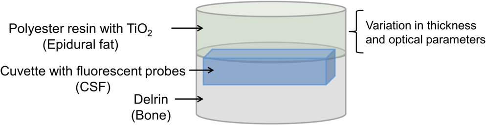

2.5.

Reference Phantom

A reference phantom required for the calibration process was composed of polyester resin with titanium dioxide, similar to the slabs used for the multilayered phantom. The thickness of the phantom was 3.1 mm, with a 1.26% titanium dioxide mass percentage.

2.6.

Ex Vivo Tissue

In order to verify the method’s accuracy in a medium that better mimics the human tissue optical properties, especially absorption, the method was further tested using chicken breast tissues. A 0.2 mL tube with a fluorescent sample was placed between two slabs of chicken breast tissue. Each slab had a nonuniform thickness varying between 2 and 8 mm. The total thickness of the set of chicken slabs with the tube in between did not exceed 14 mm. Four sets were prepared, containing tubes with fluorescent probes in different concentration ratios.

2.7.

System Setup

The samples were excited with a mode-locked, Ti:sapphire femtosecond laser (Tsunami, Spectra-Physics Lasers), with an 80 MHz repetition rate, pumped by a 5 W, 532 nm laser (Millenia Vs., Spectra-Physics Lasers). The laser was tuned to 750 nm for the Cy7 excitation and 800 nm for the Cy7.5 excitation. The excitation beam was split to a fast photodiode (PHD-400, Becker & Hickl GmbH) for signal synchronization and to the center of a fluorescence inspection fiber bundle (Oriel 77558, Newport), which illuminated the phantoms. Fluorescent photons were collected by the outer fibers of the bundle encountering a filter wheel switching between a band-pass filter FF01-780/12 (Semrock) for the Cy7 and long-pass filters RG830 and RG850 (Newport) for the Cy7.5 collection. The emission was measured using a fast photomultiplier tube (PMT) head (H7422P-50, Hamamatsu). The PMT was controlled using the DCC-100 detector controller (Becker & Hickl GmbH). Data acquisition was accomplished using the time correlated single photon counting (TCSPC) module (SPC-730, Becker & Hickl GmbH) synchronizing between the SYNC signal arriving from the photodiode and the constant fraction discriminator signal from the PMT.

2.8.

In Vitro and Ex Vivo Experiments

2.8.1.

Calibration process

A calibration process was performed prior to the in vitro measurements of the multilayered phantoms and the ex vivo chicken tissue measurements. For the calibration process of the first set of phantom experiments, three fluorescent samples were prepared in the following concentration ratios: $1 ∶ 2.3$ , $1 ∶ 3.7$ , and $1 ∶ 6.4$ . In order to improve the accuracy in the following sets of experiments, the number of samples used for the calibration was increased to five, covering ratios between $1 ∶ 2$ and $1 ∶ 18$ . The samples were placed in sealed cuvettes and the reference phantom was placed above them. The fluorescence energy emitted by these samples was measured in two excitation wavelengths, one for each fluorophore, with the appropriate emission filter. For each measurement, the total number of photons measured by the TCSPC system was used as the fluorescence energy value. A calibration curve of fluorescence energy ratio versus concentration ratio was created based on these measurements.

2.8.2.

Intensity ratio measurements—in vitro

Two sets of in vitro measurements were performed on fluorescent samples covering ratios between $1 ∶ 2$ and $1 ∶ 14$ using the multilayered phantoms. The first set of experiments included 8 samples and the second included 7 samples, with a total of 15 samples with different concentration ratios. Each sample was placed in the Delrin layer cavity, and several fluorescence measurements were taken. The measurements were taken using different polyester slabs with varying thicknesses and scattering coefficients placed above the samples. The fluorescence measurements were performed in both excitation wavelengths and the fluorescence energy ratio was calculated for each set of sample and polyester slab. Using the calibration curve, the measured energy ratio was converted to a concentration ratio value, which was compared to the true concentration ratio value.

2.8.3.

Intensity ratio measurements—ex vivo

Following a calibration process similar to Sec. 2.8.1, four additional fluorescent samples were prepared, covering ratios between $1 ∶ 3$ and $1 ∶ 16$ . The samples were placed between two slabs of chicken breast tissue. The fluorescence measurements were performed similar to the phantom experiments and repeated several times for each sample. The location of the fiber bundle on the tissue slab surface was changed for each excitation in order to test varying thicknesses of the nonuniform chicken slab. The measured energy ratio was converted to a concentration ratio value using the calibration curve and compared to the true concentration ratio value.

2.8.4.

Intensity time-resolved measurements

The fluorescence intensity time-resolved curve of a Cy7 sample was measured using the TCSPC system. The Cy7 sample was placed in the Delrin layer cavity with different polyester slabs with varying thicknesses and scattering coefficients placed above it.

3. Results and Discussion

3.1.

Monte Carlo Simulations

The ratio between the radiated energy and the detected fluorescence energy was between $0.5 \times 10^{- 6}$ and $30 \times 10^{- 6}$ in all simulated cases. These results indicate that a laser pulse with a power of a few dozens of milliWatts will suffice to detect the fluorescence signal in vivo when using a highly sensitive detector such as the one used in the TCSPC system.

3.2.

Intensity Ratio Experiments—In Vitro Experiments

A calibration process was performed prior to the intensity ratio measurements in order to assess the relation between the fluorescence intensity ratio and the concentration ratio. For minimizing the time required for the calibration, the first set of measurements included only three samples. Based on Eq. (1), a linear relation between the fluorescence intensity ratio and the concentration ratio was assumed.³⁵ These results were previously reported,³⁵ indicating higher errors in the high concentration ratios than in the low ratios. In order to improve the accuracy, in the following set of experiments, the calibration was performed on five samples covering a larger range of concentration ratios. In addition, the relation between the fluorescence intensity ratio and the concentration ratio was more accurately assumed to follow Eq. (2). The second-order polynomial relation presented in Eq. (2) was used for the calibration curve of both set of experiments.

The intensity ratio experiments included a total of 120 measurements performed on the multilayered phantoms. Fifteen fluorescent samples varying in their concentration ratio were measured, with eight different polyester slabs varying in their thickness and scattering coefficient. Figure 3 presents the estimated concentration ratio versus the true concentration ratio. Each data point is the average estimated value of eight measurements using eight different polyester slabs, with its 90% confidence interval. The dotted and dash-dotted lines in Fig. 3 represent the true ratio values with 5 and 10% errors, respectively. The mean absolute error of the 15 estimated values presented in Fig. 3 is 4.4%, with a standard deviation of 2.5%. The median of the absolute errors of estimation was 5.2% with a maximal absolute error of 7.85%.

Fig. 3

The estimated concentration ratio as a function of the true concentration ratio, for the multilayered phantoms experiments. The solid line represents the true ratio values. The star symbols represent the average estimated ratios with their 90% confidence interval. The dotted lines represent the true ratio values with 5% errors and the dash-dotted lines represent the true ratio values with 10% errors.

For further understanding the causes for ratio estimation errors, the errors were compared to the effective attenuation of each phantom. The effective attenuation was defined as the following product:

Eq. (3)

Effective attenuation = μ_{eff} \cdot l,

where

μ_{eff}

is the effective attenuation coefficient of the phantom according to the diffusion model [

μ_{eff} = \sqrt{3 μ_{a} (μ_{a} + μ_{s}^{'})}

],

l

is the phantom thickness,

μ_{a}

is the absorption coefficient, and

μ_{s}^{'}

is the reduced scattering coefficient.

Figure 4 presents the mean error of the estimated concentration ratio as a function of the effective attenuation. The mean error of estimation as a function of the effective attenuation was then fitted to a curve with the form of:

Eq. (4)

f (μ_{eff} \cdot l) = a \cdot μ_{eff} \cdot l \cdot \exp (b \cdot μ_{eff} \cdot l) + c .

Fig. 4

The mean error of estimated concentration ratio (star symbols) with their 90% confidence interval, as a function of the phantoms effective attenuation. The dashed line represents the diffusion model fit performed on the presented data. The solid line represents a zero error, and the circle symbol represents the effective attenuation of the reference phantom, expected to have a zero error.

The curve is presented by the dashed line in Fig. 4.

This function is proportional to the Green function describing the steady-state fluence rate as a response to an isotropic source in an infinite medium:

Eq. (5)

Φ (r) = \frac{1}{4 π D r} \exp (- μ_{eff} r),

where

D = 1 / 3 (μ_{a} + μ_{s}^{'})

is the diffusion coefficient and

r

is the distance from source.

According to this fit, the error in the estimated concentration ratio is negative for the high effective attenuation values due to underestimation of the concentration error. In the lower effective attenuation values, there was an overestimation of the concentration ratios causing a positive mean error. The circle symbol in Fig. 4 represents the effective attenuation value of the reference phantom used for the calibration, which was expected to have a zero error. The calibration curve was created based on measurements performed on a reference phantom with a certain thickness and effective attenuation. Therefore, the error is expected to be close to zero when using phantoms or tissues with similar effective attenuations. However, when estimating the concentration ratio for tissues or phantoms with lower or higher effective attenuation values, the errors tend to increase. These errors are caused by neglecting the energy loss caused by the photon propagation in the tissue in the ratio calculation in Eq. (1). The energy loss is neglected since it is assumed that the scattering and absorption are similar for both wavelengths and the ratio cancels both energy losses. However, there are some slight differences in the scattering and absorption coefficients of the tissue or phantom between both wavelengths. These slight differences might cause some minor errors when estimating the concentration ratio. The concentration ratio estimation from the fluorescence energy ratio is based on a calibration curve created for a media that may differ in its thickness and/or optical properties. Figure 4 demonstrates this phenomenon, where the concentration ratios were overestimated for low effective attenuation phantoms since there were less energy losses than assumed by the calibration. On the other hand, for the phantoms with higher effective attenuation values, the energy losses were higher than expected. Therefore, the concentration ratio was underestimated with some negative errors. For all cases, the absolute mean error was $< 5.5 %$ , with an average of 3.34% and the standard deviation of the absolute mean errors was 1.8%.

3.3.

Intensity Ratio Experiments—Ex Vivo Experiments

The absorption spectra of the polyester phantoms are rather flat in the 750 to 800 nm range³⁹ compared to the human tissue absorption spectra. In order to better simulate the variations in the human spectra, the method was tested using four sets of ex vivo samples of chicken tissue. Prior to the measurements performed on the chicken tissue, a calibration process was performed using the same polyester reference phantom as in the previous section. The calibration curve was used for estimation of the concentration ratios of the fluorescent probes located in between the chicken tissue slabs. Figure 5 presents the estimated concentration ratio versus the true concentration ratio. Each data point is the average estimated value of four measurements (performed on different excitation locations on the nonuniform tissue slab) with its 90% confidence interval. The dash-dotted line in Fig. 5 represents the true ratio values with 15% error. The mean absolute error of the estimated values presented in Fig. 5 is 10.9%, with a standard deviation of 7.8%. In most cases, the estimated value was higher than the true concentration ratio. This result indicates that the effective attenuation of the tissue slab was lower than the effective attenuation of the polyester slab due to less scattering and absorption coefficients and/or lower thickness of the tissue. However, in some cases, the concentration ratio was underestimated, probably when the excitation was performed on thick areas of the tissue.

Fig. 5

The estimated concentration ratio as a function of the true concentration ratio for the chicken tissue experiments. The solid line represents the true ratio values. The star symbols represent the average estimated ratios with their 90% confidence interval. The dash-dotted lines represent the true ratio values with 15% errors.

When comparing the in vitro and ex vivo results, it is evident that the accuracy in the in vitro experiments is higher than the ex vivo. The reduction in the accuracy in the ex vivo tissues may be explained by several reasons. First, the reference phantom was similar to the phantoms used in the in vitro results, thus sharing the same scattering and absorption spectra. These spectra differ from the scattering and absorption spectra of the chicken tissue. Since the calibration curve is based on the phantom measurements, these differences cause some inaccuracies in the ratio calculation. These inaccuracies may be reduced by choosing for the calibration a phantom that better resembles the tissue spectra. In addition, if the thickness of the reference phantom is significantly lower or higher than the measured tissue, the concentration ratio estimation will suffer from additional inaccuracies. Therefore, having some information regarding the distance from the fluorescent probes could assist in choosing a suitable phantom. This information may be provided by measuring time-resolved fluorescence, as will be presented in the following section.

3.4.

Intensity Time-Resolved Experiments

The fluorescence intensity was measured using the TCSPC system, which provides the fluorescence intensity time-resolved curves. The time-resolved curves were further analyzed in order to assess a feedback system for the needle location. The feedback system aims to avoid penetration of the dura layer into the CSF and reduce the risks and side effects of the lumbar puncture process. Since the time-resolved intensity curves contain information regarding the photon path length, which can easily be extracted, these measurements may be used for such a feedback system. In order to verify that the information regarding the needle location may be easily estimated, two features were extracted from each curve. The first feature is $t_{\max}$ , which represents the time in which the intensity reached its maximal value. The second feature is the slope of the decaying part of the intensity curve, in logarithmic scale. These two features were calculated for two sets of polyester slabs with two scattering coefficients and a variety of thicknesses. Figure 6 demonstrates the extracted features for three cases: (1) low-scattering polyester slab with a thickness of 2.7 mm, (2) low-scattering polyester slab with a thickness of 4 mm, and (3) high-scattering polyester slab with a thickness of 4 mm. The changes in the two features due to the thickness and scattering coefficient of the polyester phantom slab may be noticed in this figure.

Fig. 6

The time-resolved intensity curve for three cases: (1) low-scattering polyester slab with a thickness of 2.7 mm presented by the solid line; (2) low-scattering polyester slab with a thickness of 4 mm, presented by the dashed line; (3) high-scattering polyester slab with a thickness of 4 mm, presented by the dotted line. The time of the maximal intensity ( $t_{max}$ ) and the slope of the decaying curves for the three cases are marked.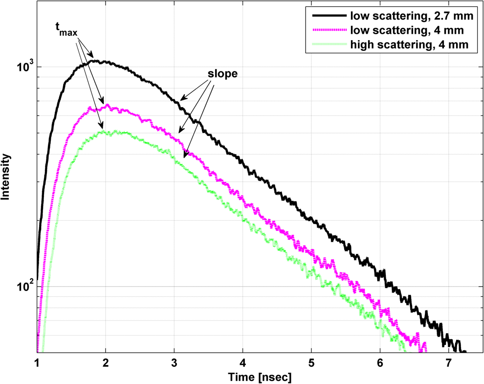

The value of $t_{\max}$ represents the time required for most of the photons to reach the detector and is related directly to the photon path length and the fluorophores depth.⁴⁰^,⁴¹ The photon path length is affected both by the scattering coefficient and the thickness of the phantom. In order to accurately estimate the effect of each one of these on $t_{\max}$ and the slope of the decaying curve, the analysis was separated for the high-scattering coefficient and the low-scattering coefficient. Figure 7(a) presents the extracted values of $t_{\max}$ as a function of the polyester phantom thickness for the low- and high-scattering coefficients. As expected, the value of $t_{\max}$ increases with an increase in the phantom thickness. This is due to the larger photon path length required until the fluorescent photons reach the detector. In addition, higher-scattering coefficients cause more scattering events, which increase the photon path length and the time value in which the intensity reaches its maximal value. A linear regression was performed on the data, with better fit results for the low-scattering phantoms ( $R^{2} = 0.96$ ) than for the high-scattering phantoms ( $R^{2} = 0.92$ ). The small reduction in the quality of fit in the high-scattering case is probably due to the lower intensity of the signal in these phantoms than in the low-scattering phantoms. The intensity is lower since the path length of photons traveling in high-scattering media increases, thus reducing the energy reaching the detector compared to low-scattering media. Therefore, the signal-to-noise ratio in the high-scattering cases is lower and the accuracy of the extracted features is lower.

Fig. 7

(a) The extracted values of $t_{max}$ as a function of the polyester phantom thickness. (b) The extracted values of intensity decay slope (absolute value) as a function of the polyester phantom thickness. In both figures, the low-scattering phantoms are presented with the square symbols and the high-scattering phantoms with the circle symbols. The linear fit performed on the low-scattering data is presented with the solid line, and the linear fit performed on the high-scattering data is presented with the dashed line.

The slope of the linear fit performed on the data presented in Fig. 7(a) was compared to the scattering coefficient. According to the diffusion model, for large distances, $t_{\max}$ is linearly dependent on the distance from source:⁴²

Eq. (6)

t_{\max} = \frac{r}{2 c} \sqrt{3 μ_{s}^{'} / μ_{a}},

where

c

is the speed of light in the medium and

r

is the distance from the source (represented by the phantom thickness).

Assuming that the absorption coefficient is similar in all phantoms, the slope of Fig. 7(a) should be proportional to the square root of the reduced scattering coefficient. In order to verify this relation, the slope of each of the two fits, the small and large scattering, was divided by $\sqrt{μ_{s}^{'}}$ . As expected, the quotients were similar for both scattering coefficients with a value of $0.013 \pm 0.0004$ .

Figure 7(b) presents the second extracted feature—the absolute value of the slope of the decaying intensity as a function of the phantom thickness for the cases of low and high scattering. As demonstrated in this figure, the absolute value of the slope of the decaying intensity curve decreases with an increase in the phantom thickness. In other words, there is a steeper decline in the intensity in thin phantoms compared to the thicker phantoms. When comparing the slope of the low and high scattering, one can notice that the high-scattering phantoms have a smaller absolute slope than the low-scattering phantoms for a given phantom thickness. In both cases, high-scattering and thick phantoms, there are more scattering events causing more photons to arrive at later times, thus reducing the absolute slope of the intensity decay curve. A linear regression was performed on the data, with slightly better fit results for the low-scattering phantoms ( $R^{2} = 0.996$ ) than for the high-scattering phantoms ( $R^{2} = 0.985$ ). Similar to the $t_{\max}$ fitting, since the low-scattering phantoms yielded a higher signal-to-noise ratio, the fit results were slightly better.

The suggested method for concentration ratio measurements of the biomarkers in the CSF involves an insertion of a needle into the lumbar section. Multiple intensity time-resolved measurements may be taken either by using multiple fibers in the same needle or by a single fiber in multiple depths during the needle insertion. According to Boon et al.,⁸ there is a distance of $\sim 5 cm$ between the skin and the epidural space, and an additional average distance of 7 mm until reaching the dura and the CSF.⁸ Therefore, an initial time-resolved intensity measurement may be taken when a sufficient signal is detected, with an additional measurement taken several millimeters deeper. Such a scheme will provide two time-resolved intensity curves (or even more) taken from a known distance between them. The values of $t_{max}$ and the slope will then be extracted from these two curves, enabling accurate estimation of the absolute value of the needle distance from the CSF. The needle distance is estimated without a priori knowledge of the tissue optical properties. Such information provided in real time may be used as a feedback system. This system will assist in preventing penetration of the dura and reducing injuries, complications, and side effects, which are common in the lumbar puncture process. The accuracy of the estimated needle distance from the CSF may be increased by using photon propagation models for multilayered tissues. Such models enable extraction of anatomical information and optical properties estimation from the time-resolved intensity curves.⁴³^–⁴⁵

4. Conclusions

The proposed method for optical detection of AD using fluorescent probes in the CSF was verified with Monte Carlo simulations, in vitro, and ex vivo experiments. The in vitro and ex vivo experiments validated the possibility to accurately estimate the ratio between amyloid-beta and tau proteins in the CSF. The method does not require any a priori knowledge regarding the tissue anatomical and optical properties and is performed without the need to penetrate the dura and collect CSF samples. In addition, a feedback system for the needle location was presented, which can assist in avoiding any complication and risks involved in such a procedure.

This simple nonionizing, low-risk method aims to detect AD up to nine years earlier than present exams. Its accuracy is expected to be high, similar to the studies where the CSF was drawn in a lumbar puncture. Our proposed method may be used as an annual screening test to assist in the diagnosis of the disease in its early stage and help treat it effectively. It has the potential to reduce medical healthcare costs, improve the quality of life of many patients, and may even save lives.

Acknowledgments

Osnat Harbater acknowledges the support of the Israeli Ministry of Science and Technology and the support of the Herczeg Institute on Aging for this research.

References

1.

“2014 Alzheimer’s disease facts and figures,” Alzheimer’s Dementia, 10 (2), e47 –e92 (2014). http://dx.doi.org/10.1016/j.jalz.2014.02.001 1552-5260 Google Scholar

2.

P. J. NestorP. ScheltensJ. R. Hodges, “Advances in the early detection of Alzheimer’s disease,” Nat. Rev. Neurosci., 5 S34 –S41 (2004). http://dx.doi.org/10.1038/nrn1433 NRNAAN 1471-0048 Google Scholar

3.

O. Hanssonet al., “Association between CSF biomarkers and incipient Alzheimer’s disease in patients with mild cognitive impairment: a follow-up study,” Lancet Neurol., 5 (3), 228 –234 (2006). http://dx.doi.org/10.1016/S1474-4422(06)70355-6 LNAEAM 1474-4422 Google Scholar

4.

N. Andreasenet al., “Cerebrospinal fluid levels of total‐tau, phospho‐tau and Aβ42 predicts development of Alzheimer’s disease in patients with mild cognitive impairment,” Acta Neurol. Scand., 107 (s179), 47 –51 (2003). http://dx.doi.org/10.1034/j.1600-0404.107.s179.9.x ANRSAS 0001-6314 Google Scholar

5.

P. Buchhaveet al., “Cerebrospinal fluid levels of {beta}-amyloid 1-42, but not of tau, are fully changed already 5 to 10 years before the onset of Alzheimer dementia,” Arch. Gen. Psychiatry, 69 (1), 98 (2012). http://dx.doi.org/10.1001/archgenpsychiatry.2011.155 ARGPAQ 0003-990X Google Scholar

6.

L. M. Shawet al., “Biomarkers of neurodegeneration for diagnosis and monitoring therapeutics,” Nat. Rev. Drug Discov., 6 (4), 295 –303 (2007). http://dx.doi.org/10.1038/nrd2176 NRDDAG 1474-1776 Google Scholar

7.

L. M. Shawet al., “Cerebrospinal fluid biomarker signature in Alzheimer’s disease neuroimaging initiative subjects,” Ann. Neurol., 65 (4), 403 –413 (2009). http://dx.doi.org/10.1002/(ISSN)1531-8249 ANNED3 0364-5134 Google Scholar

8.

J. Boonet al., “Lumbar puncture: anatomical review of a clinical skill,” Clin. Anat., 17 (7), 544 –553 (2004). http://dx.doi.org/10.1002/(ISSN)1098-2353 CLANE8 1098-2353 Google Scholar

9.

J. W. Mcmurdyet al., “Noninvasive optical, electrical, and acoustic methods of total hemoglobin determination,” Clin. Chem., 54 (2), 264 –272 (2008). http://dx.doi.org/10.1373/clinchem.2007.093948 CLCHAU 0009-9147 Google Scholar

10.

T. C. ZhuJ. C. FinlayS. M. Hahn, “Determination of the distribution of light, optical properties, drug concentration, and tissue oxygenation in-vivo in human prostate during motexafin lutetium-mediated photodynamic therapy,” J. Photochem. Photobiol. B: Biol., 79 (3), 231 –241 (2005). http://dx.doi.org/10.1016/j.jphotobiol.2004.09.013 JPPBEG 1011-1344 Google Scholar

11.

A. Leprouxet al., “Assessing tumor contrast in radiographically dense breast tissue using diffuse optical spectroscopic imaging (DOSI),” Breast Cancer Res., 15 (5), R89 (2013). http://dx.doi.org/10.1186/bcr3485 BCTRD6 1465-5411 Google Scholar

12.

E. Sevick-Muraca, “Translation of near-infrared fluorescence imaging technologies: emerging clinical applications,” Annu. Rev. Med., 63 217 –231 (2012). http://dx.doi.org/10.1146/annurev-med-070910-083323 ARMCAH 0066-4219 Google Scholar

13.

F. Leblondet al., “Pre-clinical whole-body fluorescence imaging: review of instruments, methods and applications,” J. Photochem. Photobiol. B: Biol., 98 (1), 77 –94 (2010). http://dx.doi.org/10.1016/j.jphotobiol.2009.11.007 JPPBEG 1011-1344 Google Scholar

14.

A. SoubretJ. RipollV. Ntziachristos, “Accuracy of fluorescent tomography in the presence of heterogeneities: study of the normalized Born ratio,” IEEE Trans. Med. Imaging, 24 (10), 1377 –1386 (2005). http://dx.doi.org/10.1109/TMI.2005.857213 ITMID4 0278-0062 Google Scholar

15.

M. SinaasappelH. Sterenborg, “Quantification of the hematoporphyrin derivative by fluorescence measurement using dual-wavelength excitation and dual-wavelength detection,” Appl. Opt., 32 (4), 541 –548 (1993). http://dx.doi.org/10.1364/AO.32.000541 APOPAI 0003-6935 Google Scholar

16.

V. NtziachristosR. Weissleder, “Charge-coupled-device based scanner for tomography of fluorescent near-infrared probes in turbid media,” Med. Phys., 29 (5), 803 (2002). http://dx.doi.org/10.1118/1.1470209 MPHYA6 0094-2405 Google Scholar

17.

E. E. Graveset al., “Validation of in vivo fluorochrome concentrations measured using fluorescence molecular tomography,” J. Biomed. Opt., 10 (4), 044019 (2005). http://dx.doi.org/10.1117/1.1993427 JBOPFO 1083-3668 Google Scholar

18.

J. LeeE. M. Sevick-Muraca, “Three-dimensional fluorescence enhanced optical tomography using referenced frequency-domain photon migration measurements at emission and excitation wavelengths,” JOSA A, 19 (4), 759 –771 (2002). http://dx.doi.org/10.1364/JOSAA.19.000759 JOAOD6 1084-7529 Google Scholar

19.

A. GodavartyE. M. Sevick-MuracaM. J. Eppstein, “Three-dimensional fluorescence lifetime tomography,” Med. Phys., 32 (4), 992 (2005). http://dx.doi.org/10.1118/1.1861160 MPHYA6 0094-2405 Google Scholar

20.

B. YuanQ. Zhu, “Separately reconstructing the structural and functional parameters of a fluorescent inclusion embedded in a turbid medium,” Opt. Express, 14 (16), 7172 –7187 (2006). http://dx.doi.org/10.1364/OE.14.007172 OPEXFF 1094-4087 Google Scholar

21.

A. Joshiet al., “Radiative transport-based frequency-domain fluorescence tomography,” Phys. Med. Biol., 53 (8), 2069 (2008). http://dx.doi.org/10.1088/0031-9155/53/8/005 PHMBA7 0031-9155 Google Scholar

22.

V. Chernomordiket al., “Inverse method 3-D reconstruction of localized in vivo fluorescence—application to Sjogren syndrome,” IEEE J. Sel. Topics Quantum Electron., 5 (4), 930 –935 (1999). http://dx.doi.org/10.1109/2944.796313 IJSQEN 1077-260X Google Scholar

23.

A. Eidsathet al., “Three-dimensional localization of fluorescent masses deeply embedded in tissue,” Phys. Med. Biol., 47 (22), 4079 (2002). http://dx.doi.org/10.1088/0031-9155/47/22/311 PHMBA7 0031-9155 Google Scholar

24.

I. Gannotet al., “In vivo quantitative three-dimensional localization of tumor labeled with exogenous specific fluorescence markers,” Appl. Opt., 42 (16), 3073 –3080 (2003). http://dx.doi.org/10.1364/AO.42.003073 APOPAI 0003-6935 Google Scholar

25.

I. Gannotet al., “Quantitative optical imaging of the pharmacokinetics of fluorescent-specific antibodies to tumor markers through tissuelike turbid media,” Opt. Lett., 29 (7), 742 –744 (2004). http://dx.doi.org/10.1364/OL.29.000742 OPLEDP 0146-9592 Google Scholar

26.

C. D’Andreaet al., “Localization and quantification of fluorescent inclusions embedded in a turbid medium,” Phys. Med. Biol., 50 (10), 2313 (2005). http://dx.doi.org/10.1088/0031-9155/50/10/009 PHMBA7 0031-9155 Google Scholar

27.

S.-H. HanS. Farshchi-HeydariD. J. Hall, “Analytical method for the fast time-domain reconstruction of fluorescent inclusions in vitro and in vivo,” Biophys. J., 98 (2), 350 –357 (2010). http://dx.doi.org/10.1016/j.bpj.2009.10.008 BIOJAU 0006-3495 Google Scholar

28.

D. J. Hallet al., “In vivo simultaneous monitoring of two fluorophores with lifetime contrast using a full-field time domain system,” Appl. Opt., 48 (10), D74 –D78 (2009). http://dx.doi.org/10.1364/AO.48.000D74 APOPAI 0003-6935 Google Scholar

29.

S. B. Raymondet al., “Lifetime-based tomographic multiplexing,” J. Biomed. Opt., 15 (4), 046011 (2010). http://dx.doi.org/10.1117/1.3469797 JBOPFO 1083-3668 Google Scholar

30.

S. B. Raymondet al., “Smart optical probes for near-infrared fluorescence imaging of Alzheimer’s disease pathology,” Eur. J. Nucl. Med. Mol. Imaging, 35 (Suppl. 1), 93 –98 (2008). http://dx.doi.org/10.1007/s00259-007-0708-7 EJNMA6 1619-7070 Google Scholar

31.

M. Hintersteineret al., “In vivo detection of amyloid-β deposits by near-infrared imaging using an oxazine-derivative probe,” Nat. Biotechnol., 23 (5), 577 –583 (2005). http://dx.doi.org/10.1038/nbt1085 NABIF9 1087-0156 Google Scholar

32.

C. Ranet al., “Design, synthesis, and testing of difluoroboron-derivatized curcumins as near-infrared probes for in vivo detection of amyloid-β deposits,” J. Am. Chem. Soc., 131 (42), 15257 –15261 (2009). http://dx.doi.org/10.1021/ja9047043 JACSAT 0002-7863 Google Scholar

33.

N. Okamuraet al., “In vivo detection of amyloid plaques in the mouse brain using the near-infrared fluorescence probe THK-265,” J. Alzheimers Dis., 23 (1), 37 –48 (2011). http://dx.doi.org/10.3233/JAD-2010-100270 JADIF9 1387-2877 Google Scholar

34.

A. Bashkatovet al., “Optical properties of human skin, subcutaneous and mucous tissues in the wavelength range from 400 to 2000 nm,” J. Phys. D: Appl. Phys., 38 (15), 2543 (2005). http://dx.doi.org/10.1088/0022-3727/38/15/004 JPAPBE 0022-3727 Google Scholar

35.

O. HarbaterI. Gannot, “Measurement of fluorescent probes concentration ratio in the cerebrospinal fluid for early detection of Alzheimer’s disease,” Proc. SPIE, 8940 89400U (2014). http://dx.doi.org/10.1117/12.2039043 PSISDG 0277-786X Google Scholar

36.

E. OkadaD. T. Delpy, “Near-infrared light propagation in an adult head model. I. Modeling of low-level scattering in the cerebrospinal fluid layer,” Appl. Opt., 42 (16), 2906 –2914 (2003). http://dx.doi.org/10.1364/AO.42.002906 APOPAI 0003-6935 Google Scholar

37.

P. Van Der Zee, “Measurement and modelling of the optical properties of human tissue in the near infrared,” University of London (1992). Google Scholar

38.

A. Sassaroliet al., “Time-resolved measurements of in vivo optical properties of piglet brain,” Opt. Rev., 7 (5), 420 –425 (2000). http://dx.doi.org/10.1007/s10043-000-0420-3 1340-6000 Google Scholar

39.

M. FirbankD. Delpy, “A design for a stable and reproducible phantom for use in near infra-red imaging and spectroscopy,” Phys. Med. Biol., 38 (6), 847 (1993). http://dx.doi.org/10.1088/0031-9155/38/6/015 PHMBA7 0031-9155 Google Scholar

40.

J. Rileyet al., “Choice of data types in time resolved fluorescence enhanced diffuse optical tomography,” Med. Phys., 34 (12), 4890 –4900 (2007). http://dx.doi.org/10.1118/1.2804775 MPHYA6 0094-2405 Google Scholar

41.

D. Hallet al., “Simple time-domain optical method for estimating the depth and concentration of a fluorescent inclusion in a turbid medium,” Opt. Lett., 29 (19), 2258 –2260 (2004). http://dx.doi.org/10.1364/OL.29.002258 OPLEDP 0146-9592 Google Scholar

42.

G. NishimuraM. Tamura, “Simple peak shift analysis of time-of-flight data with a slow instrumental response function,” J. Biomed. Opt., 10 (1), 014016 (2005). http://dx.doi.org/10.1117/1.1854684 JBOPFO 1083-3668 Google Scholar

43.

I. SteinbergO. HarbaterI. Gannot, “Robust estimation of cerebral hemodynamics in neonates using multilayered diffusion model for normal and oblique incidences,” J. Biomed. Opt., 19 (7), 071406 (2014). http://dx.doi.org/10.1117/1.JBO.19.7.071406 JBOPFO 1083-3668 Google Scholar

44.

A. LiemertA. Kienle, “Light diffusion in N-layered turbid media: frequency and time domains,” J. Biomed. Opt., 15 (2), 025002 (2010). http://dx.doi.org/10.1117/1.3368682 JBOPFO 1083-3668 Google Scholar

45.

J.-M. Tualleet al., “Asymptotic behavior and inverse problem in layered scattering media,” J. Opt. Soc. Am. A, 21 (1), 24 –34 (2004). http://dx.doi.org/10.1364/JOSAA.21.000024 JOAOD6 0740-3232 Google Scholar

Biography

Osnat Harbater received her BSc degree in biomedical engineering from the Technion-Israeli Institute of Technology, Israel, in 2004 and her MSc degree in biomedical engineering in Tel-Aviv University, Israel, in 2011. She is currently pursuing her PhD degree in biomedical engineering in Tel-Aviv University, Israel. Her research interests include photon propagation models in tissue, developing novel optical methods for diagnosing Alzheimer's disease, monitoring cerebral hemodynamics, and optical imaging modalities for additional medical applications.

Israel Gannot received his PhD degree from Tel-Aviv University in 1994. Between 1994 and 1997, he held a National Academy Sciences postdoctoral fellowship. Since 1997, he is a member of the Biomedical Engineering Department at the Tel-Aviv University where he served as a chair. Currently, he is also a research professor at Johns Hopkins University. He is a fellow of SPIE, ASLMS, and AIMBE. He authored 60 papers, 90 proceeding papers, seven book chapters, and 14 patents.

Citation Download Citation

Osnat Harbater and Israel Gannot "Fluorescent probes concentration estimation in vitro and ex vivo as a model for early detection of Alzheimer’s disease," Journal of Biomedical Optics 19(12), 127007 (29 December 2014). https://doi.org/10.1117/1.JBO.19.12.127007

Published: 29 December 2014

Access the abstract

JOURNAL ARTICLE
9 PAGES

DOWNLOAD PAPER SAVE TO MY LIBRARY

GET CITATION

CITATIONS

Cited by 6 scholarly publications.

Explore citations on Lens.org

RIGHTS & PERMISSIONS

Get copyright permission Get copyright permission on Copyright Marketplace

KEYWORDS

Luminescence

Tissues

Scattering

In vitro testing

Calibration

Signal attenuation

Absorption

1.

Introduction

Fig. 1

2.

Methods

2.1.

Model and Assumptions

Eq. (1)

Eq. (2)

2.2.

Monte Carlo Simulations

2.3.

Fluorescent Probes

2.4.

Multilayered Phantoms

Fig. 2

2.5.

Reference Phantom

2.6.

Ex Vivo Tissue

2.7.

System Setup

2.8.

In Vitro and Ex Vivo Experiments

2.8.1.

Calibration process

2.8.2.

Intensity ratio measurements—in vitro

2.8.3.

Intensity ratio measurements—ex vivo

2.8.4.

Intensity time-resolved measurements

3.

Results and Discussion

3.1.

Monte Carlo Simulations

3.2.

Intensity Ratio Experiments—In Vitro Experiments

Fig. 3

Eq. (3)

Eq. (4)

Fig. 4

Eq. (5)

3.3.

Intensity Ratio Experiments—Ex Vivo Experiments

Fig. 5

3.4.

Intensity Time-Resolved Experiments

Fig. 6

Fig. 7

Eq. (6)

4.

Conclusions

Acknowledgments

References

Biography

Show All Keywords

Keywords/Phrases

Search In:

Publication Years