Three-dimensional counting of morphologically normal human red blood cells via digital holographic microscopy

Faliu Yi; Inkyu Moon; Yeon  H. Lee

doi:10.1117/1.JBO.20.1.016005

7 January 2015 Three-dimensional counting of morphologically normal human red blood cells via digital holographic microscopy

Faliu Yi, Inkyu Moon, Yeon H. Lee

Author Affiliations +

Journal of Biomedical Optics, Vol. 20, Issue 1, 016005 (January 2015). https://doi.org/10.1117/1.JBO.20.1.016005

Abstract

Counting morphologically normal cells in human red blood cells (RBCs) is extremely beneficial in the health care field. We propose a three-dimensional (3-D) classification method of automatically determining the morphologically normal RBCs in the phase image of multiple human RBCs that are obtained by off-axis digital holographic microscopy (DHM). The RBC holograms are first recorded by DHM, and then the phase images of multiple RBCs are reconstructed by a computational numerical algorithm. To design the classifier, the three typical RBC shapes, which are stomatocyte, discocyte, and echinocyte, are used for training and testing. Nonmain or abnormal RBC shapes different from the three normal shapes are defined as the fourth category. Ten features, including projected surface area, average phase value, mean corpuscular hemoglobin, perimeter, mean corpuscular hemoglobin surface density, circularity, mean phase of center part, sphericity coefficient, elongation, and pallor, are extracted from each RBC after segmenting the reconstructed phase images by using a watershed transform algorithm. Moreover, four additional properties, such as projected surface area, perimeter, average phase value, and elongation, are measured from the inner part of each cell, which can give significant information beyond the previous 10 features for the separation of the RBC groups; these are verified in the experiment by the statistical method of Hotelling’s T-square test. We also apply the principal component analysis algorithm to reduce the dimension number of variables and establish the Gaussian mixture densities using the projected data with the first eight principal components. Consequently, the Gaussian mixtures are used to design the discriminant functions based on Bayesian decision theory. To improve the performance of the Bayes classifier and the accuracy of estimation of its error rate, the leaving-one-out technique is applied. Experimental results show that the proposed method can yield good results for calculating the percentage of each typical normal RBC shape in a reconstructed phase image of multiple RBCs that will be favorable to the analysis of RBC-related diseases. In addition, we show that the discrimination performance for the counting of normal shapes of RBCs can be improved by using 3-D features of an RBC.

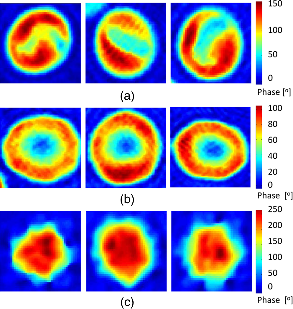
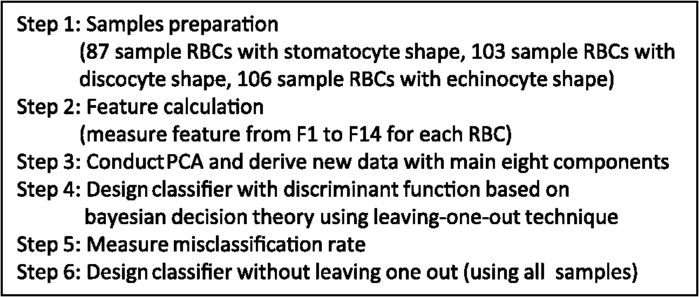
1. Introduction

The three-dimensional (3-D) holographic imaging system has been studied for visualization, identification, and tracking of biological micro/nano-organisms.¹^–⁶ In the areas of biomedical imaging, defense, medical diagnosis, medical therapeutics, and security, the 3-D holographic imaging system has a lot of potential.¹^–⁹

Red blood cells (RBCs), which are the principal method of delivering oxygen to body tissues via the blood flowing through the circulatory system in vertebrate organisms, are the most common type of blood cell. RBCs are also an imperative part of human beings because they absorb oxygen in the lungs and release it when squeezing through the body’s capillaries.¹⁰ Therefore, RBCs have been extensively studied for biomedical applications with the development of new technology and equipment.¹¹^–¹⁶ Recent studies have demonstrated that patients suffer from latent risk when RBCs stored for a substantial amount of time or having abnormal shapes are transfused into the patients’ bodies because the function and viability of RBCs are disorderedly changed;¹⁷ such changes can affect other body tissues indirectly.¹⁸^,¹⁹ Therefore, it is extremely important to have a classification algorithm that can categorize different types of RBCs effectively and efficiently in order to overcome the shortage of the traditional method that is time-consuming and labor-intensive. In addition, counting cell types in the blood is an important task for evaluating clinical status. In this paper, three main types of RBC shapes, stomatocyte, discocyte, and echinocyte,²⁰^–²³ are defined and used for the quantitative determination of the percentage of morphologically normal cell shapes in multiple human RBCs. Without a doubt, the RBC with the discocyte shape accounts for the majority of RBCs in a normal human, and the percentage of other RBC types varies between healthy and nonhealthy individuals. Scientists can also predict that, for a variety of RBC-related diseases, the percentages of different types of RBCs will be distinct.²³ Furthermore, under the effects of specific drugs or agents, the structure and function of RBCs can be modified. Thus, it will be helpful to measure the percentage of typical normal shapes of RBCs in a reconstructed RBC phase image that consists of multiple RBCs for disease diagnosis and drug testing. Admittedly, in addition to the three typical types of RBCs, there are other types of RBCs. Therefore, nonmain or abnormal RBC shapes that are different from the three normal shapes are defined as the fourth category. If an RBC is classified into the fourth class, it means that the confidence level of grouping the RBC into the three typical types is low.

In this paper, the RBC holograms are captured by off-axis digital holographic microscopy (DHM) and the RBC phase images are reconstructed through the computational numerical algorithm.²⁴^,²⁵ These phase images are proportional to the cellular thickness; therefore, they can provide 3-D structural information of the RBCs. Consequently, the RBC phase images can compensate for the limitation received from intensity images obtained by conventional two-dimensional (2-D) imaging systems. Although some advanced 2-D imaging systems, such as quantitative phase contrast and differential interference contrast microscopes, can quantitatively investigate biological microorganisms, they cannot provide important optical thickness information regarding the cells.²⁶ Moreover, off-axis digital holographic imaging systems can achieve high contrast images for semitransparent/transparent targets without destruction of the specimen, which is different from conventional microscopy such as electron microscopy.²³ In our previous works, we have shown that a single RBC can be extracted from a reconstructed phase image with multiple RBCs²⁷ in DHM system. Moreover, we experimentally demonstrate that joint statistical distributions of the characteristic parameters of RBCs can be obtained using two kinds of RBCs (stomatocyte and discocyte shape RBCs).²⁸ In Ref. 10, the authors also successfully demonstrated that it is possible to classify and recognize RBCs based on their storage duration using DHM. However, the method based on a clustering approach results in a high misclassification rate, particularly for RBCs with a long storage period.

For classification of different types of RBCs in this paper, the discriminant functions based on Bayesian decision theory, which can realize minimum-error-rate classification, is adopted.²⁹ First, 10 features, including projected surface area, average phase value, mean corpuscular hemoglobin (MCH), perimeter, MCH surface density (MCHSD), circularity, mean phase of center part, sphericity coefficient, elongation, and pallor (phase value difference between cell edge and center), are extracted from each RBC after segmenting the reconstructed phase images through an edge-based segmentation method (the watershed algorithm³⁰ is used in our paper). In addition, four more features, such as projected surface area, perimeter, average phase value, and elongation, are measured from the inner part of each segmented RBC and can provide significant information in grouping the RBCs beyond the previous 10 features. This is verified through the statistical method of Hotelling’s $T$ -square test in our experiment. Next, the principal component analysis (PCA) algorithm²⁹^,³⁰ is applied to all 14 features in order to reduce the dimension space. Thus, the original data can be projected onto a low dimension space using 60% of the primary components, and the mixture Gaussian densities can be established with the projected data when we assume that they follow the multivariate Gaussian distribution. Accordingly, the Gaussian mixtures are used to design the discriminant functions based on Bayesian decision theory.²⁹^,³¹ In this experiment, we have extracted 87 samples of stomatocyte shape, 103 samples of discocyte shape, and 106 samples of echinocyte shape and analyzed them to design the classifier. Because the simple separation of the samples into training and testing sets limits the accuracy of both the training and the testing phases of the pattern classifier design,²⁹ we apply the leaving-one-out technique²⁹^,³¹ to our samples, which nearly doubles the effective size of the sample data. Experimental results show that the classifier obtained by our method gives a good performance in counting automatically the morphologically normal cells in multiple human RBCs. In addition, we demonstrate that the discrimination performance for the counting of normal shapes of RBCs can be enhanced by using the 3-D features of an RBC.

This paper is organized as follows. Section 2 describes the preparation of the RBCs that are analyzed in our experiment and the principle of the off-axis DHM that is utilized to capture the 3-D RBC images. Section 3 presents the concept of Bayesian decision theory and the leaving-one-out technique. Section 4 describes the classifier design procedures to automatically count the morphologically normal cells in multiple RBCs. The experimental results are provided in Sec. 5. Finally, the conclusion is presented in Sec. 6.

2. RBC Preparation and Off-Axis DHM

2.1.

RBC Preparation

The RBCs of healthy laboratory personnel were obtained through the Laboratoire Suisse d’ Analyse Du Dopage—CHUV and stored at 4°C during the storage period. The DHM measurements were performed several days after the blood was collected from the laboratory personnel. A total of 100 to $150 μ l$ of RBC stock solution were suspended in a high-efficiency particulate air (HEPA) buffer (15 mM 2-[4-(2-hydroxyethyl) piperazin-1-yl] ethanesulfonic acid, pH 7.4, 130 mM NaCl, 5.4 mM KCl, 10 mM glucose, 1 mM ${CaCl}_{2}$ , 0.5 mM ${MgCl}_{2}$ , and $1 mg / ml$ bovine serum albumin) at 0.2% hematocrit for predominantly stomatocyte and discocyte shaped RBCs while at a concentration of $\sim 0.15 %$ for predominantly echinocyte shaped RBCs. A total of $4 μ l$ of the erythrocyte suspension were diluted to $150 μ l$ of the HEPA buffer and introduced into the experimental chamber, including two cover slips separated by spacers 1.2-mm thick. The cells were incubated for 30 min at a temperature of 37°C before mounting on the chamber on the DHM stage. All experiments were performed at room temperature (22°C).

2.2.

Off-Axis DHM

The off-axis DHM imaging system described in Ref. 32, which is a modified Mach–Zehnder configuration with off-axis geometry, is used in our implementation. A laser diode source with $λ = 682 nm$ is used in the 3-D imaging system. Then the laser beam is separated into a reference wave and an object wave. When the object wave passes through the RBC samples, it is diffracted and magnified by a $40 \times / 0.75$ numerical aperture microscope objective. The diffracted object wave interferes with the reference wave in the off-axis geometry. Consequently, the interference pattern is recorded via a charge-coupled device camera. For the reconstruction and aberration compensation of the RBC wave front, the computational numerical algorithm described in Refs. 24 and 25 is used. The resolution of the RBC phase images reconstructed from the hologram is $704 \times 704$ in our experiment. Figure 1 shows some reconstructed phase images of the sample RBCs with stomatocyte, discocyte, and echinocyte shapes, respectively. They are the three main RBC shapes that will be used in our classifier design. In our definition, the stomatocyte RBC shape has a narrow central part, whereas the discocyte RBC shape has a rather circular central area. For RBCs with an echinocyte shape, there is no apparent central region and the phase value of the central part is also high compared with other areas.

Fig. 1

Reconstructed red blood cell (RBC) phase images: (a) stomatocyte RBC shape, (b) discocyte RBC shape, and (c) echinocyte RBC shape.

3. Bayesian Decision Algorithm and Leaving-One-Out Technique

In this section, we describe the concept of Bayesian decision algorithm and leaving-one-out technique. The Bayesian decision algorithm, which belongs to the statistical decision-making technique, is used to design a pattern classifier using a training set with known classes.³²^,³³ The leaving-one-out method is a type of cross-validation technique²⁹ that can improve the performance of the designed classifier and the accuracy of the estimation of error rate.

3.1.

Bayesian Decision Algorithms

The Bayesian decision algorithm is a type of statistical decision-making approach for the problem of pattern classification. The probability of a pattern belonging to a specific class is the combination of a prior probability and a likelihood probability that can be expressed as Eq. (1) with one feature and $n$ classes²⁹^,³³

Eq. (1)

P (C_{i} | x) = \frac{p (x | C_{i}) p (C_{i})}{p (x)},

where

p (x) = p (x | C_{1}) p (C_{1}) + p (x | C_{2}) p (C_{2}) + \dots + p (x | C_{n}) p (C_{n})

is viewed as a scale factor such that the summation of the posterior probabilities

p (C_{i} | x)

is equal to one or can be used as a constant,

p (C_{i})

is the a priori probability that represents the probability that class

i

appears among all the populations, whereas the conditional probability

p (x | C_{i})

is the likelihood that denotes the probability of feature

x

occurring in a given class

C_{i}

, and

n

is the number of classes. Consequently, the posterior probabilities

p (C_{i} | x)

that represents the probability of a given feature

x

to be classified into a specific class

i

can be derived by the basic Bayes theorem in Eq. (1). Most of the time, a single feature is not enough to discriminate the classes. Multiple features are a better choice to distinguish the classes in a high dimension. The Bayes theorem for multiple features can be expressed as Eq. (2), which is similar to Eq. (1), but replaces the single feature

x

with a feature vector

x

, including multiple features, and the likelihood

p (x | C_{i})

is a joint conditional probability (for discrete cases):

Eq. (2)

P (C_{i} | x) = \frac{p (x | C_{i}) p (C_{i})}{p (x) = \sum_{j = 1}^{n} p (x | C_{j}) p (C_{j})} .

For the pattern classifiers based on the Bayesian decision theory, the discriminant functions that are represented as

g_{i} (x)

, where

i = 1, \dots, n

denotes the

i

’th class are widely used. For a sample with multiple features

x

, when

g_{i} (x) > g_{j} (x)

and

i \neq j

, the sample is classified into class

C_{i}

that corresponds to the class with the highest posterior probability in the Bayes theorem. Thus, the discriminant functions can be achieved through Eq. (3):

Eq. (3)

g_{i} (x) = P (C_{i} | x) = \frac{p (x | C_{i}) p (C_{i})}{p (x) = \sum_{j = 1}^{n} p (x | C_{j}) p (C_{j})} .

Because

p (x)

does not affect the decision and can be viewed as a constant, the denominator in Eq. (3) can be eliminated. In order to simplify the discriminant function so that it is much easier to understand, the discriminant function can be written in a simpler form as shown in Eq. (4) by taking the natural logarithm of the numerator in Eq. (3):

Eq. (4)

g_{i} (x) = \ln p (x | C_{i}) + \ln p (C_{i}) .

As a result, the discriminant function based on the Bayesian decision theory is determined by the conditional probabilities (likelihood) $p (x | C_{i})$ and a priori probabilities $p (C_{i})$ . In particular, when the multiple features satisfy the multivariate normal distribution, the conditional probabilities can be described by the multivariate normal density shown in Eq. (5):²⁹

Eq. (5)

p (x | C_{i}) = \frac{1}{{(2 π)}^{d / 2} {| \sum_{i} |}^{1 / 2}} \exp [- \frac{1}{2} {(x - μ_{i})}^{t} \sum_{i}^{- 1} (x - μ_{i})],

where

x

is a

d

-dimensional feature column vector,

μ_{i}

is the

d

-dimensional mean vector of the

i

’th class,

\sum_{i}

is the

d

-by-

d

dimensional covariance matrix of the

i

’th class, and

| \sum_{i} |

and

\sum^{- 1}

are the determinant and inverse of covariance matrix, respectively. Consequently, the discriminant function in Eq. (4) can be easily evaluated as Eq. (6) if the conditional probabilities are a mixture Gaussian distribution [replace

p (x | C_{i})

in Eq. (4) with Eq. (5)]:

Eq. (6)

g_{i} (x) = - \frac{1}{2} {(x - μ_{i})}^{t} \sum_{i}^{- 1} (x - μ_{i}) - \frac{d}{2} \ln 2 π - \frac{1}{2} \ln | \sum_{i} | + \ln p (C_{i}) .

Thus, the features are categorized into the class that can achieve the largest discriminant value. The discriminant function derived from the Bayesian decision theory is proven to be able to achieve the minimum-error-rate among all the classifiers.²⁹^,³³

3.2.

Leaving-One-Out Technique

It is evident that a classifier designed with as many training and testing sets as possible is much more robust in terms of improving the classifier performance and the accuracy for estimating its error rate. However, because of the limited number of the available sample data, the accuracy of both the training and testing classifier is restricted. The leaving-one-out method is a type of technique that can avoid the previous limitation to a large extent because this approach nearly doubles the effective size of the sample data.²⁹ The procedure of the leaving-one-out technique is described as follows. Suppose that $n$ samples are provided in the data set; the classifier obtained by leaving-one-out is not designed and is investigated simply by dividing the samples into the training and testing sets not at one time, but at $n$ times. In this process, one sample from the data set is withdrawn from the testing set and the other $n - 1$ samples are used to design the classifier. Thus, the withheld sample can be tested by the classifier designed with the $n - 1$ samples. This is logical because the classifier is designed without this particular sample. The previous step can be repeated $n$ times and each time a different testing sample is omitted; thus, all $n$ samples are used as the testing set. For each round, a new classifier is established with $n - 1$ samples and tested by the one sample that is omitted in the design of the classifier. Consequently, the expected probability of error can be deduced as $k / n$ on an average classifier that is trained on the $n - 1$ samples; $k$ is the number of errors in the testing phase. Because the samples in this technique are prevented from being in both the training and the testing of a given classifier, the error rate estimate can be regarded as unbiased and accurate because all the samples are used for testing.²⁹ Finally, the classifier is designed using the total $n$ samples as training, and its expected error rate is at least as low as $k / n$ because the classifier is created with $n$ samples, but not with the $n - 1$ samples used in the leaving-one-out step. This process is illustrated in Fig. 2. Step 1 in Fig. 2 is conducted $n$ times until no new sample can be used as the test sample. The classifier $g_{i} (x)$ is designed based on Bayesian decision algorithm. After the table shown in step 2 of Fig. 2 is achieved, the misclassification rate can be measured. Finally, all of the samples are applied to design the classifier, which will be used to predict the sample with an unknown class.

Fig. 2

Flowchart of leaving-one-out technique.

4. Classifier Design Procedures

In this procedure, after the RBC phase images are reconstructed using the computational numerical algorithm from the holograms obtained through the off-axis DHM, each RBC is extracted with the background removed by the watershed transform segmentation approach.³⁰ Then the 10 features listed in Table 1 are calculated from each segmented whole RBC. In addition, in order to increase the performance of separating the RBC groups, four more features, including projected surface area, perimeter, average phase value, and elongation are measured from the inner part of the segmented RBCs; these are also presented in Table 1. The segmented whole and the inner part of an RBC are illustrated in Fig. 3.

Table 1

Description of 14 features.

Segmented whole RBC
Feature	Description
F1: projected surface area	Number of pixels within single $RBC \times 1 pixel$ area
F2: perimeter	Cell boundary length
F3: circularity	$(Perimeter \times perimeter) / area$
F4: average phase value	Average phase value for pixels within single RBC
F5: MCH	Mean corpuscular hemoglobin
F6: MCHSD	MCH surface density
F7: phase of center pixel	Center pixel phase value (average $5 \times 5 pixels$ )
F8: sphericity coefficient	Center part phase value/maximal phase value
F9: elongation	Chain code orientation in cell boundary
F10: $D$ -value	Center pixel phase value minus maximum pixel phase value
Inner part of segmented RBC
F11: projected surface area	Number of pixels within inner part of $RBC \times 1 pixel$ area
F12: perimeter	Boundary length in inner part of cell
F13: average phase value	Average phase value for pixels within inner part of RBC
F14: elongation	Chain code orientation in boundary of inner part of cell

Fig. 3

Illustration of segmented whole cell and inner part of cell.

The projected surface area, average phase value, MCH, and MCHSD are calculated from each segmented whole RBC as shown in Eq. (7):

Eq. (7)

S = N \frac{p^{2}}{M^{2}}, \bar{φ} = \frac{1}{N} \sum_{i = 1}^{N} φ_{i}, MCH = \frac{10 λ}{2 π α} S \bar{φ}, MCHSD = \frac{MCH}{S},

where

N

is the number of pixels within a single RBC,

p

is the pixel size,

M

is the magnification of the DHM,

φ_{i}

is the phase value at the

i

’th pixel within a single RBC,

λ

is the wavelength of the light source, and

α

, known as the specific refraction increment, is a constant. When the boundary of each cell is marked by an eight-directional Freeman chain code,³⁰^,³⁴ the perimeter, circularity, and elongation features can be achieved as shown in Eq. (8):³⁴

Eq. (8)

perimeter = N_{e} \times 1 + N_{o} \times \sqrt{2}, circularity = {perimeter}^{2} / area, elongation = \max (| N_{0,4} - N_{2,6} |, | N_{1,5} - N_{3,7} |), N_{j, k} = \underset{a_{i = j} or a_{i = k}}{\sum_{i = 1}^{n}} 1,

where

N_{e}

is the number of even-valued elements, whereas

N_{o}

is the number of odd elements in the boundary chain code of a single RBC, and

n

(

= N_{e} + N_{o}

) is the total number of elements in the Freeman chain code for each RBC. In addition, the phase value of the center pixel is defined as the average phase value of the central

5 \times 5 pixels

, the sphericity coefficient is the division between the phase value of the center pixel and the maximum phase value within each segmented whole RBC, and the

D

-value is the difference between the phase value in the center pixel and the maximum phase value. To measure the four features in the inner part of an RBC, the previous equations can be used repeatedly when only these features of the inner part need to be determined instead of the segmented whole cell.

Here, we apply the statistical method of Hotelling’s $T$ -square test³⁵ to show that the features calculated from the inner part of the cell can, indeed, provide additional separation between RBC groups beyond the separation already achieved by the 10 features obtained from the segmented whole cell. Let $y$ denote the $p \times 1$ vector where $p = 10$ includes the 10 variables used to measure the features in the segmented cell; furthermore, let $x$ denote the $q \times 1$ vector where $q = 4$ expresses the four variables used to calculate the properties in the segmented inner part of the cell. We assume that each pair of samples is from the multivariate normal population and that $x_{1}$ and $x_{2}$ are two $q \times 1$ vectors, whereas $y_{1}$ and $y_{2}$ are two $p \times 1$ vectors from two different groups. Then the null hypothesis [ $H_{0}$ : $x_{1}$ and $x_{2}$ are redundant for separating the two classes beyond $y_{1}$ and $y_{2}$ ] can be represented as shown in Eq. (9):³⁵

Eq. (9)

T^{2} (x | y) = (v - p) \frac{T_{p + q}^{2} - T_{p}^{2}}{v + T_{p}^{2}},

which is distributed as

T_{q, v - p}^{2}

where

v = n_{1} + n_{2} - 2

, whereas

n_{1}

and

n_{2}

are the number of samples in the two groups, respectively. When

T^{2} (x | y) \geq T_{α, q, v - p}^{2}

, the null hypothesis

H_{0}

that

x

is redundant is rejected at a significance level of

α

where the critical value of

T_{α, q, v - p}^{2}

can be achieved from the

T^{2}

-table with

q

and

v - p

degrees of freedom. For Eq. (9),

T_{p + q}^{2}

and

T_{p}^{2}

are expressed, respectively, as Eqs. (10) and (11):³⁵

Eq. (10)

T_{p + q}^{2} = \frac{n_{1} n_{2}}{n_{1} + n_{2}} {[(\frac{{\bar{y}}_{1}}{{\bar{x}}_{1}}) - (\frac{{\bar{y}}_{2}}{{\bar{x}}_{2}})]}^{'} {(\begin{matrix} S_{y y} & S_{y x} \\ S_{x y} & S_{x x} \end{matrix})}^{- 1} [(\frac{{\bar{y}}_{1}}{{\bar{x}}_{1}}) - (\frac{{\bar{y}}_{2}}{{\bar{x}}_{2}})],

Eq. (11)

T_{p}^{2} = \frac{n_{1} n_{2}}{n_{1} + n_{2}} {({\bar{y}}_{1} - {\bar{y}}_{2})}^{'} S_{y y}^{- 1} ({\bar{y}}_{1} - {\bar{y}}_{22}),

where

{\bar{y}}_{1}

and

{\bar{y}}_{2}

are the sample mean vectors, and

S_{y y}

,

S_{y x}

, and

S_{x x}

are the covariance matrices. In the experimental section, we present the

T^{2}

statistic test results among each pair of RBC groups.

In order to demonstrate that 3-D features of an RBC extracted from DHM imaging technique are beneficial to distinguish different kinds of RBCs, we divide the RBC’s features into two categories that are given in Table 2. One is defined as 2-D features, which can be acquired from the 2-D imaging system and the other is defined as 3-D features, which are obtained from the DHM technique. Then, the Hotelling’s $T$ -square test, as per the previous description for inner part feature analysis, is conducted to check whether the 3-D features can provide additional separation among RBCs classes beyond the partition already achieved by the 2-D features. In this case, $x$ in Eq. (9) denotes the seven features from the 2-D features category and $y$ represents the other seven features from the 3-D features group.

Table 2

Division of RBC features.

2-D features	F1, F2, F3, F9, F11, F12, F14
3-D features	F4, F5, F6, F7, F8, F10, F13

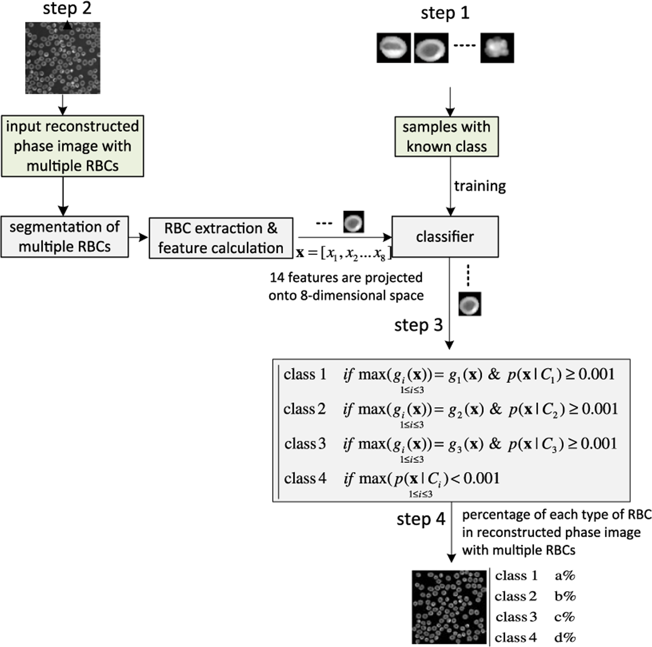
In our experiment, we use 87 RBCs labeled as stomatocyte shape, 103 RBCs labeled as discocyte shape, and 106 RBCs labeled as echinocyte shape. In addition, the total 14 features denoted by the feature vector as ${[X_{1} X_{2} \dots X_{14}]}^{t}$ in each RBC are calculated. It should be noted that when there are no inner parts for certain RBCs, a random value from the standard normal distribution is assigned to the features from F11 to F14 in Table 1. The samples with the known class that is used to design the classifier are listed in Fig. 4.

Fig. 4

Samples used to train classifier.

After all the 14 properties are determined from the samples, the PCA algorithm is applied to these features to reduce the variable dimension; we retained 60% of the principal components, that is, eight components, for the classifier design in the next step. Consequently, the original data can be projected onto an eight-dimensional space using the eight principal components. Here, we assume that all of the data obtained satisfy the multivariate normal distribution. Accordingly, the joint density [conditional probability in Eq. (2)] of the multiple features for each type of RBC can be represented by a mixture of Gaussian density as expressed in Eq. (5) with features after being projected from the eight principal components. Furthermore, we can assume that the a priori probabilities [ $p (C_{i})$ in Eq. (6)] for each class are equal so that this term can be removed from the discriminant function as well as the constant term $0.5 d \ln 2 π$ because they do not affect the pattern classification in this case. Therefore, the discriminant function in Eq. (6) based on Bayesian decision theory can be further simplified as shown in Eq. (12):

Eq. (12)

g_{i} (x) = - \frac{1}{2} {(x - μ_{i})}^{t} \sum_{i}^{- 1} (x - μ_{i}) - \frac{1}{2} \ln | \sum_{i} | 1 \leq i \leq 3,

where

μ_{i}

and

\sum_{i}

are estimated from their respective sample data using an unbiased estimator.²⁹ Consequently, one type of RBC corresponds to one discriminant function and three discriminant functions are required for the classification of three classes of RBCs (class 1: stomatocyte shape RBCs, class 2: discocyte shape RBCs, and class 3: echinocyte shape RBCs). The testing pattern is categorized into the class that can achieve the largest value for the corresponding discriminant function. Considering the situation where there are other types of RBC in addition to the three typical types of RBCs, the fourth class, which includes all types of RBCs excluding these three typical classes, is defined. When the probability of one sample belonging to any one of the three typical types of RBCs is low, it is grouped into the fourth class. This can be achieved by Eq. (5) because the discriminant function in Eq. (3) is proportional to the value of the likelihood [Eq. (5)] that the a priori probability is assumed to be the same for all types of RBCs. In this paper, when the density in the likelihood [Eq. (5)] of the extracted features from an RBC is

< 0.001

among all the three typical types of RBCs, we classify the corresponding RBC into the fourth class. The flowchart for our classifier design and RBC classification is presented in Fig. 5.

Fig. 5

Flowchart of RBC classification.

First, the classifier is designed based on the Bayesian design theory by the leaving-one-out technique with the samples from the known class (step 1 in Fig. 5). Then the obtained classifier is used to categorize the RBCs in a reconstructed phase image with multiple RBCs (step 2 in Fig. 5). In this step, the original RBC phase images and the inner part of the RBCs have to be segmented to extract all the RBCs and calculate the corresponding features.

Subsequently, all the RBCs in the reconstructed RBC phase images are grouped into the four types of RBCs as described in Fig. 5. Finally, the percentage of the different types of RBCs in the RBC phase images can be calculated and analyzed (step 4 in Fig. 5). In particular, when the occupation ratio of the fourth class reaches the highest value in a reconstructed RBC phase image, this image should be further examined carefully because this situation is not normal for a healthy person. The leaving-one-out technique for improving the design of the classifier and for estimating the error rate is implemented by the pseudocode shown in Fig. 6 (based on MATLAB). For the final design of the classifiers [class 1 denoted as $g_{1} (x)$ , class 2 denoted as $g_{2} (x)$ , and class 3 denoted as $g_{3} (x)$ ], all the sample data are used as a training set.

Fig. 6

Pseudocode for the leaving-one-out test.

5. Experimental Results

The simulation and measurement in this paper are all executed on a 32-bit Windows 7 computer with a 3.30 GHz Intel Core i5-2500 CPU, 4 GB RAM, and 4 cores. The RBC phase images are reconstructed using the computational numerical algorithm from the holograms obtained by the off-axis DHM; then, the phase images are segmented by the watershed transform algorithm. The reconstructed phase images, segmented RBCs, and the segmented inner part of the RBCs are shown in Fig. 7 with the three typical types of RBCs. After segmentation, all the 14 features are measured. Table 3 lists the quantitative validation for the extracted 14 features.

Fig. 7

Reconstructed RBC phase images and their segmented phase images. (a), (b), and (c) are the reconstructed phase images for predominantly stomatocyte, discocyte, and echinocyte shape RBCs, respectively. (d), (e), and (f) are the corresponding segmented phase images from (a), (b), and (c). (g), (h), and (i) are the segmented inner part of the RBCs in (a), (b), and (c).

Table 3

Quantitative validation of calculated 14 features from samples.

Features	RBCs with stomatocyte shape (87 samples)		RBCs with discocyte shape (103 samples)		RBCs with echinocyte shape (106 samples)
Features	Mean	Std	Mean	Std	Mean	Std
F1	34.31	3.83	47.28	5.40	25.76	3.96
F2	21.96	1.30	25.36	1.58	18.83	1.73
F3	14.13	0.44	13.67	0.37	13.84	0.93
F4	97.75	12.58	67.55	10.13	136.86	16.77
F5	31.60	4.12	30.10	5.01	33.04	4.29
F6	0.92	0.11	0.65	0.08	1.29	0.15
F7	84.35	28.21	26.84	14.41	207.70	37.73
F8	0.50	0.11	0.24	0.12	0.91	0.10
F9	7.73	5.32	8.38	5.73	6.12	4.75
F10	81.88	24.07	88.70	25.60	23.21	20.41
F11	9.83	3.36	20.50	4.43	0.01	0.93
F12	12.61	2.43	17.03	1.94	0.08	0.83
F13	81.50	11.65	56.72	7.72	0.10	0.97
F14	12.13	6.25	7.30	5.69	0.06	1.03

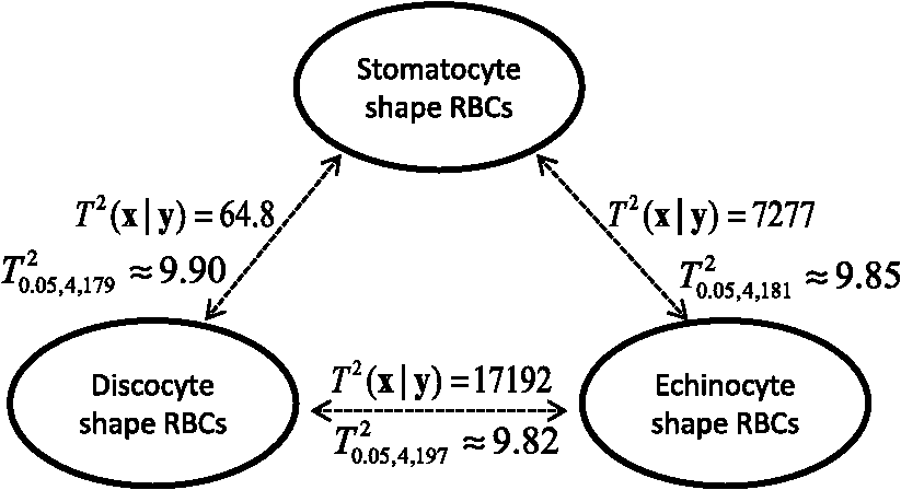
In our experiment, we have demonstrated that the features from the inner part of the RBCs are not redundant, but can contribute information to the separation of the RBC groups by Hotelling’s $T$ -square test. The calculated $T^{2} (x | y)$ value and critical value of $T_{α, q, v - p}^{2}$ (see Sec. 4 for details) searched from the $T^{2}$ -table are shown in Fig. 8. It is noted that all the $T^{2} (x | y)$ values among each pair of RBC groups are larger than their corresponding critical value. Consequently, we reject the null hypothesis $H_{0}$ when the features from the inner part of the RBCs are not significant in separating the RBC groups at the 0.05 level of significance. In other words, the features from the inner part of the RBCs can be helpful in classifying the RBCs. Similarly, statistical analysis results shown in Fig. 9 reveal that 3-D features of an RBC extracted from the DHM imaging system can contribute to separating the RBCs classes. Therefore, the discrimination performance for counting normal shapes of RBCs can be improved by adding to the 3-D features of an RBC to the 2-D ones.

Fig. 8

Redundance analysis results for inner part features of RBCs with Hotelling’s $T$ -square test.

Fig. 9

Redundance analysis results for three-dimensional (3-D) features (see Table 2) of RBCs with Hotelling’s $T$ -square test.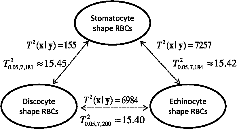

Next, the PCA algorithm is applied to the 14 features, and 60% of the principal components (that is eight principal components) are retained to design the Bayesian-based classifier. Because we assume that the multiple variables satisfy the multivariate Gaussian distribution, the mixture Gaussian density of each group can be established by the features obtained from the multiplication of the original sample features with the extracted eight principal components. Therefore, the corresponding discriminant function can be realized with the created mixture Gaussian density for each RBC population as Eq. (12). As the design presented in Fig. 6, the leave-one-out experiment results show that the misclassification rate for the RBCs with stomatocyte shape is $3 / 87 = 3.45 %$ , the misclassification rate for the RBCs with discocyte shape is $4 / 103 = 3.88 %$ , and the misclassification rate for the RBCs with echinocyte shape is $3 / 106 = 2.83 %$ . On the contrary, the misclassification rates for RBCs with stomatocyte, discocyte, and echinocyte shapes only using 2-D features (see Table 2) are measured to be $11 / 87 = 12.64 %$ , $13 / 103 = 12.62 %$ , and $6 / 106 = 5.66 %$ , respectively. It is noted that the classifier based on the Bayesian decision algorithm with both 2-D and 3-D features achieved a very good result for the classification of RBCs with three different shapes. This demonstrates that the discrimination performance for classification of different types of RBCs can be enhanced by using the 3-D features of an RBC. Moreover, the throughput, which is defined as the processed data per second in our method, is measured to be $27.64 Mb / s$ and the total computational time for the training and testing process is calculated to be 0.0024 s by averaging the simulation results of 20 times.

The results of analyzing the percentage of morphologically normal RBCs in the reconstructed phase images with multiple RBCs are also shown in Fig. 10. Figures 10(a), 10(b), and 10(c) are the measured percentages of the typical normal shapes of RBCs in the reconstructed RBC phase images. It is visually found that the majority of RBCs in each RBC’s phase image are consistent with the highest percentage rate for the corresponding image in Fig. 10. These percentages are automatically derived from the classifier that is obtained by our classifier algorithm whose misclassification rates are demonstrated to be low. We believe that the proposed classifier can be adopted to automatically count the morphologically normal cells in multiple human RBCs. In addition, the classifier can be helpful for the analysis of RBC-related diseases because the occupation ratio of the different types of RBCs is associated with certain types of diseases.

Fig. 10

Analysis of reconstructed phase image with multiple RBCs. (a), (b), and (c) are the segmented images with percentages of each type of RBC labeled by our designed classifier method. (Class 1: RBCs with stomatocyte shape, class 2: RBCs with discocyte shape, class 3: RBCs with echinocyte shape, and class 4: other types of RBC).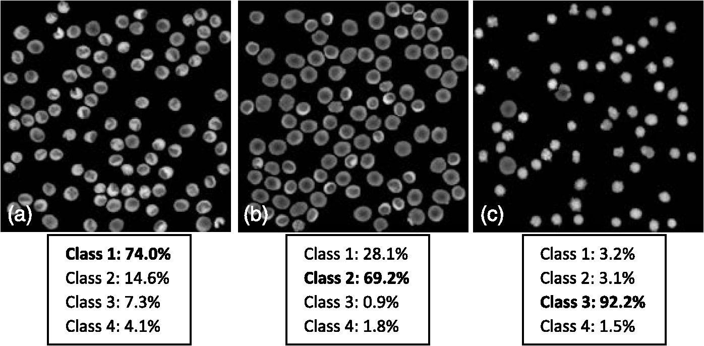

6. Conclusion

In this paper, we designed a classifier using DHM and Bayesian decision theory for the automatic counting of the morphologically normal RBCs of stomatocyte, discocyte, and echinocyte shapes, which allows us to quantitatively determine the percentage of normal cell shapes in multiple human RBCs. The hologram patterns of the RBCs were first captured by the off-axis DHM, and the RBC phase images were reconstructed through the computational numerical algorithm. Ten patterns were calculated from each RBC that was extracted from the RBC phase images through the watershed transform segmentation method, and four more features were collected from the inner part of the RBC. Hotelling’s $T$ -square test showed that the features from the inner part of the RBC can significantly improve the separation of different RBC groups. In order to reduce the dimension space of the variables, the PCA algorithm was adopted, and the first eight principal components were retained to retrieve new projected features to establish the mixture Gaussian densities for each type of RBC. Subsequently, the discriminant function based on Bayesian decision theory was used to design the classifiers. Finally, in order to improve the accuracy for estimating the error rate of the classifier, the leaving-one-out technique was used and tested. Experimental results demonstrated that our classifier can give a good performance for the classification of RBCs with stomatocyte, discocyte, and echinocyte shapes. Their misclassification rates were at least as low as 3.45%, 3.88%, and 2.83%, respectively. In addition, we demonstrate that the discrimination performance for RBCs classification can be improved by using both 2-D and 3-D features of an RBC. Furthermore, the designed classifier was able to group an RBC into a fourth class when the 2-D and 3-D features of the RBC were extremely different from the three typical types of RBCs. This automatic RBC classification method can be extremely helpful for drug testing and for analyzing certain RBC-related diseases because the percentage of normal cell shapes in multiple human RBCs varies from disease to disease.

Acknowledgments

This research was supported by Basic Science Research Program through the National Research Foundation of Korea (NRF) funded by the Ministry of Education, Science, and Technology (NRF-2013R1A2A2A05005687 and NRF-2012R1A1A2039249). We thank Daniel Boss and Pierre Marquet from Ecole Polytechnique Fédérale de Lausanne (EPFL), Switzerland, for their help with the experiments.

References

1.

B. JavidiF. OkanoJ. Sun, 3D Imaging, Visualization, and Display Technologies, Springer, New York (2008). Google Scholar

2.

W. OstenT. BaumbachW. Juptner, “Comparative digital holography,” Opt. Lett., 27 1764 –1766 (2002). http://dx.doi.org/10.1364/OL.27.001764 OPLEDP 0146-9592 Google Scholar

3.

Y. Frauelet al., “Three dimensional imaging and display using computational holographic imaging,” Proc. IEEE, 94 636 –654 (2006). http://dx.doi.org/10.1109/JPROC.2006.870704 IEEPAD 0018-9219 Google Scholar

4.

S. Benton, Holographic Imaging, Wiley-Interscience, New York (2008). Google Scholar

5.

I. Moonet al., “Automated three dimensional identification and tracking of micro/nano biological organisms by computational holographic microscopy,” Proc. IEEE, 97 990 –1010 (2009). http://dx.doi.org/10.1109/JPROC.2009.2017563 IEEPAD 0018-9219 Google Scholar

6.

B. JavidiI. MoonS. Yeom, “Real-time 3D sensing and identification of microorganisms,” Opt. Photon. News Mag., 17 16 –21 (2006). http://dx.doi.org/10.1364/OPN.17.2.000016 OPPHEL 1047-6938 Google Scholar

7.

P. Langehanenberget al., “Autofocusing in digital holographic phase contrast microscopy on pure phase objects for live cell imaging,” Appl. Opt., 47 D176 –D182 (2008). http://dx.doi.org/10.1364/AO.47.00D176 APOPAI 0003-6935 Google Scholar

8.

J. ShengE. MalkielJ. Katz, “Digital holographic microscopy for measuring three-dimensional particle distributions and motions,” Appl. Opt., 45 3893 –3901 (2006). http://dx.doi.org/10.1364/AO.45.003893 APOPAI 0003-6935 Google Scholar

9.

I. MoonB. Javidi, “Shape tolerant three-dimensional recognition of biological microorganisms using digital holography,” Opt. Exp., 13 9612 –9622 (2005). http://dx.doi.org/10.1364/OPEX.13.009612 OPEXF 1094-4087 Google Scholar

10.

R. Liuet al., “Recognition and classification of red blood cells using digital holographic microscopy and data clustering with discriminant analysis,” J. Opt. Soc. Am. A, 28 (6), 1204 –1210 (2011). http://dx.doi.org/10.1364/JOSAA.28.001204 JOAOD6 0740-3232 Google Scholar

11.

B. Rappazet al., “Spatial analysis of erythrocyte membrane fluctuations by digital holographic microscopy,” Blood Cells Mol. Dis., 42 (3), 228 –232 (2009). http://dx.doi.org/10.1016/j.bcmd.2009.01.018 1079-9796 Google Scholar

12.

Z. Schishet al., “Digital holographic microscopy-innovative and non-destructive analysis of living cells,” Microsc. Sci. Technol. Appl. Educ., 4 1055 –1062 (2010). Google Scholar

13.

Y. JangJ. JangY. Park, “Dynamic spectroscopic phase microscopy for quantifying hemoglobin concentration and dynamic membrane fluctuation in red blood cells,” Opt. Exp., 20 (9), 9673 –9681 (2012). http://dx.doi.org/10.1364/OE.20.009673 OPEXF 1094-4087 Google Scholar

14.

N. GovS. Safran, “Red blood cell membrane fluctuations and shape controlled by ATP-induced cytoskeletal defects,” Biophysical, 88 1859 –1874 (2005). Google Scholar

15.

D. Bosset al., “Exploring red blood cell membrane dynamics with digital holographic microscopy,” Proc. SPIE, 7715 77153l (2010). http://dx.doi.org/10.1117/12.854717 PSISDG 0277-786X Google Scholar

16.

W. ReinhartS. Chien, “Red cell rheology in stomatocyte-echinocyte transformation: roles of cell geometry and cell shape,” Blood, 67 (4), 1110 –1118 (1986). BLOOAW 0006-4971 Google Scholar

17.

B. Bhaduriet al., “Optical assay of erythrocyte function in banked blood,” Sci. Rep., 4 6211 (2014). http://dx.doi.org/10.1038/srep06211 SRCEC3 2045-2322 Google Scholar

18.

J. LaurieD. WyncollC. Harrison, “New versus old blood—the debate continues,” Crit. Care, 14 130 –131 (2010). http://dx.doi.org/10.1186/cc8878 1364-8535 Google Scholar

19.

C. Kochet al., “Duration of red-cell storage and complications after cardiac surgery,” N. Engl. J. Med., 358 1229 –1239 (2008). http://dx.doi.org/10.1056/NEJMoa070403 NEJMAG 0028-4793 Google Scholar

20.

L. GeraldM. WortisR. Mukhopadhyay, “Stomatocyte-discocyte-echinocyte sequence of the human red blood cell: evidence for the bilayer-couple hypothesis from membrane mechanics,” Proc. Natl. Acad. Sci. U. S. A., 99 (26), 4457 –4461 (2002). PNASA6 0027-8424 Google Scholar

21.

K. KhairyJ. FooJ. Howard, “Shapes of red blood cells: comparison of 3D confocal images with the bilayer-couple model,” Cell. Mol. Bioeng., 1 (2–3), 173 –181 (2008). http://dx.doi.org/10.1007/s12195-008-0019-5 CMBECP 1865-5025 Google Scholar

22.

M. Battistelliet al., “Rhodiola rosea as antioxidant in red blood cells: ultrastructural and hemolytic behavior,” Eur. J. Histochem., 49 (3), 243 –254 (2005). EJHIE2 0391-7258 Google Scholar

23.

T. Tishko, Holographic Microscopy of Phase Microscopic Objects: Theory and Practice, World Scientific, Maryland (2011). Google Scholar

24.

E. CucheP. MarquetC. Depeursinge, “Simultaneous amplitude and quantitative phase contrast microscopy by numerical reconstruction of Fresnel off-axis holograms,” Appl. Opt., 38 6994 –7001 (1999). http://dx.doi.org/10.1364/AO.38.006994 APOPAI 0003-6935 Google Scholar

25.

T. Colombet al., “Automatic procedure for aberration compensation in digital holographic microscopy and application to specimen shape compensation,” Appl. Opt., 45 851 –863 (2006). http://dx.doi.org/10.1364/AO.45.000851 APOPAI 0003-6935 Google Scholar

26.

F. YiI. MoonY. H. Lee, “Extraction of target specimens from bioholographic images using interactive graph cuts,” J. Biomed. Opt., 18 (12), 126015 (2013). http://dx.doi.org/10.1117/1.JBO.18.12.126015 JBOPFO 1083-3668 Google Scholar

27.

F. Yiet al., “Automated segmentation of multiple red blood cells with digital holographic microscopy,” J. Biomed. Opt., 18 (2), 026006 (2013). http://dx.doi.org/10.1117/1.JBO.18.2.026006 JBOPFO 1083-3668 Google Scholar

28.

I. Moonet al., “Automated statistical quantification of three-dimensional morphology and mean corpuscular hemoglobin of multiple red blood cells,” Opt. Express, 20 (9), 10295 –10309 (2012). http://dx.doi.org/10.1364/OE.20.010295 OPEXFF 1094-4087 Google Scholar

29.

E. GoseR. Johnsonbaugh, Pattern Recognition and Image Analysis, Prentice Hall, New Jersey (1996). Google Scholar

30.

R. GonzalezR. Woods, Digital Imaging Processing, Prentice Hall, New Jersey (2002). Google Scholar

31.

H. NeyU. EssenR. Kneser, “On the estimation of ‘small’ probabilities by leaving-one-out,” IEEE Trans. Pattern Anal. Mach. Intell., 17 (12), 1202 –1212 (1995). http://dx.doi.org/10.1109/34.476512 ITPIDJ 0162-8828 Google Scholar

32.

P. Marquetet al., “Digital holographic microscopy: a noninvasive contrast imaging technique allowing quantitative visualization of living cells with subwavelength axial accuracy,” Opt. Lett., 30 468 –470 (2005). http://dx.doi.org/10.1364/OL.30.000468 OPLEDP 0146-9592 Google Scholar

33.

R. DudaP. HartD. Stork, Pattern Classification, Wiley-Interscience, New York (2000). Google Scholar

34.

J. BacusJ. Weens, “Automated method of differential red blood cell classification with application to the diagnosis of anemia,” J. Histochem. Cytochem., 25 514 –632 (1977). http://dx.doi.org/10.1177/25.7.330716 JHCYAS 0022-1554 Google Scholar

35.

A. Rencher, Methods of Multivariate Analysis, Wiley-Interscience, New York (2002). Google Scholar

Biography

Faliu Yi received a BE degree from Yunnan University, Kunming, China, in 2008 and an ME degree in computer engineering from Chosun University, Gwangju, Republic of Korea, in 2012, and is currently working toward the PhD degree in computer engineering from the same university. His research interests include three-dimensional (3-D) image processing, computer vision, image segmentation, object tracking, pattern recognition, and parallel computing.

Inkyu Moon received a BS degree in electronics engineering from Sungkyunkwan University, Republic of Korea, in 1996, and a PhD degree in electrical and computer engineering from the University of Connecticut in 2007. He joined Chosun University, Republic of Korea, in 2009, and is currently an associate professor at the School of Computer Engineering. His research interests include digital holography, biomedical imaging, and optical information processing. He is a member of IEEE, OSA, and SPIE.

Yeon H. Lee received a BS degree in electronics engineering from Seoul National University, Republic of Korea, in 1980, and a PhD degree in electrical engineering from the University of Southern California in 1989. He joined Sungkyunkwan University, Republic of Korea, in 1992, and is currently a professor with the Electrical Engineering Department. His research area involves holographic optical memory, image processing, encryption, and 3-D display. He is the author of the book Introduction to Engineering Electromagnetics, Springer, 2013.

Citation Download Citation

Faliu Yi, Inkyu Moon, and Yeon H. Lee "Three-dimensional counting of morphologically normal human red blood cells via digital holographic microscopy," Journal of Biomedical Optics 20(1), 016005 (7 January 2015). https://doi.org/10.1117/1.JBO.20.1.016005

Published: 7 January 2015

Access the abstract

JOURNAL ARTICLE
10 PAGES

DOWNLOAD PAPER SAVE TO MY LIBRARY

GET CITATION

CITATIONS

Cited by 37 scholarly publications.

Explore citations on Lens.org

RIGHTS & PERMISSIONS

Get copyright permission Get copyright permission on Copyright Marketplace

KEYWORDS

Image segmentation

3D image reconstruction

Blood

Digital holography

3D image processing

Shape analysis

Error analysis

1.

Introduction

2.

RBC Preparation and Off-Axis DHM

2.1.

RBC Preparation

2.2.

Off-Axis DHM

Fig. 1

3.

Bayesian Decision Algorithm and Leaving-One-Out Technique

3.1.

Bayesian Decision Algorithms

Eq. (1)

Eq. (2)

Eq. (3)

Eq. (4)

Eq. (5)

Eq. (6)

3.2.

Leaving-One-Out Technique

Fig. 2

4.

Classifier Design Procedures

Table 1

Fig. 3

Eq. (7)

Eq. (8)

Eq. (9)

Eq. (10)

Eq. (11)

Table 2

Fig. 4

Eq. (12)

Fig. 5

Fig. 6

5.

Experimental Results

Fig. 7

Table 3

Fig. 8

Fig. 9

Fig. 10

6.

Conclusion

Acknowledgments

References

Biography

Show All Keywords

Keywords/Phrases

Search In:

Publication Years