1.

Introduction

Co-registration is the process of assigning the correct anatomical locations to the points from which physiological data are recorded.¹ Anatomical localization of functional brain data is central to cognitive neuroscience and to the preoperative application of imaging methods. However, many functional brain imaging techniques measure brain activity without a concurrently recorded anatomical frame of reference and rely instead on anatomical information separately obtained through structural magnetic resonance imaging (sMRI) or computerized axial tomography.

These functional imaging techniques, which typically rely on scalp-placed recording sensors, include electroencephalography and event-related brain potentials (EEG and ERPs),^2,3 magnetoencephalography (MEG),⁴ transcranial magnetic stimulation (TMS),⁵ functional near-infrared spectroscopy (fNIRS),^6–8 and fast optical and event-related optical signals (FOS and EROS).⁹ EEG and ERPs rely on the measurement of the electromagnetic fields generated by active neurons, which are broadly volume-conducted across the scalp, limiting their spatial resolution. However, the use of high-density montages and sophisticated inverse solutions for EEG and ERPs^10,11 increases the need for accurate and stable co-registration algorithms. Optical imaging methods (fNIRS, FOS, and EROS) measure changes in the propagation of NIR light through the head tissue, which is affected by hemodynamic and neuronal activity. Functional changes in light parameters decay within a short distance (a few centimeters) from their source.¹² Thus, these measures can be strongly affected by co-registration errors, particularly when high density diffusive optical tomography (HD-DOT)¹³ is considered and depth resolution is required.

Co-registration involves aligning two data sets: an anatomical data set (typically a volumetric anatomical MR image of the brain) and a set comprising three-dimensional (3-D) measurements of the scalp locations from which the functional data were recorded (which can be obtained using a magnetic 3-D digitizer or an optical photographic method), but which may also contain additional points that are only included to facilitate the co-registration process. Typically, these two data sets are obtained separately and use different frames of reference. In addition, both can potentially contain some measurement errors, although typically only errors in the measurement of the recording locations are considered. As such, the co-registration problem can be defined as the set of procedures used to transform the coordinates of the recording locations from those based on their original frame of reference into those based on the same frame of reference used to express the anatomical information. These procedures are not trivial and require sophisticated algorithms in order to achieve the most accurate solution. In this paper, we compare procedures for co-registration, including a novel procedure called iterative closest point-to-plane (ICP2P), to provide guidelines about their application.

A common method to co-register anatomical and functional data is to determine a set of anatomical landmarks, or fiducial points^14,15 that are identified and tagged both on the anatomical image and on the sensor-placement framework. If we do not consider measurement error, a simple system of linear equations can then be used to co-register the fiducial points’ coordinates obtained from the 3-D digitizer onto the corresponding points of the anatomical image. To solve the co-registration equations, a minimum of three noncolinear fiducial points is needed. By convention and for reliability across labs, fiducial points typically include the two preauricular points and the nasion, which were used as reference markers in the 10-20 system for EEG/ERP electrode placement.¹⁶ These same fiducial locations continue to be used for EEG/ERP electrode positioning and have also been used as reference points for co-registering the head to the MEG dewar¹⁷ and TMS data onto anatomical MRIs.¹⁸ More accurate but invasive transcutaneous markers have been used for preoperative clinical procedures and can sometimes provide submillimeter precision.^15,19,20 The main advantages of fiducial alignment are the simplicity of the co-registration algorithm, its negligible computational time, and the fact that it does not require a description of the entire scalp surface, but only a few specific points.

A major disadvantage of fiducial alignment is that it can be significantly affected by errors in replicating the placement of the fiducials across the two measurement sessions (i.e., scalp sensor digitization and anatomical imaging, respectively). Since the method described above depends on a deterministic (i.e., not statistical) model, it does not include the possibility of error, therefore, there is no procedure to minimize its effects. Using a larger number of fiducials and applying a statistical model can ameliorate the problem. However, there is little agreement on how many fiducial points are needed to produce optimal results. Further, methods based on fiducials require time to accurately digitize the points on the subject and to identify and place markers over these same points for MRI. Last, fiducial alignment is limited to points that can be identified reliably across multiple sessions. Thus, only a few fiducials are typically used and these are normally located in the front or on the side of the head. This means that the co-registration of posterior locations, as well as of locations placed above or below the plane identified by the three fiducial points, need to be based on extrapolation, a process that is likely to significantly decrease co-registration accuracy.

Surface-fitting procedures^21–24 offer alternative or supplemental methods to fiducial-based approaches. They fit a discrete sampling of two surfaces, one represented by the digitized points and another represented by points extracted from a rendition of the scalp derived from an sMRI image. Fitting means finding the regression parameters (i.e., a set of three values related to the translation of the two surfaces so that they are co-centered, and a set of three angles used to rotate the two surfaces so that they are oriented in the same direction) that minimize an error term (also called objective function). This problem is nonlinear, as it involves angles, therefore, it has no simple analytical solution. As such, the problem is addressed by an iterative method that explores the space defined by the possible angles, looking for a point in this space (i.e., a combination of the various parameters) that minimizes the objective function. Each iteration involves three steps: (1) a guess about the values of the parameters; (2) the computation of the resulting value of the objective function (or error); and (3) a strategy used to move to another guess. The iterative procedure is interrupted when the error does not reduce anymore with further iterations (stop rule).

A problem with this method is that there is no guarantee that it will find the correct solution. It is possible that other combinations of parameters that were never explored could produce an error value that is even better than the one observed. This problem is typically minimized if the initial guess (i.e., the guess used at the first iteration) is relatively close to the correct solution. Alternatively, the method used to search the parameter space should be sufficiently reliable so as to eliminate this possibility. Another problem (common to all regression methods) is that various solutions may produce very similar errors and that the difference between them (which is also subject to sampling error) may not be large enough to ensure that the one chosen is really superior to the others (this is equivalent to saying that the confidence interval for a particular estimate is very large and that little confidence should be put on any particular solution). This problem may be generated by a poor sampling strategy, one that does not provide a detailed enough description of the two surfaces to be fit.

Four factors will, therefore, determine the accuracy of surface-fitting procedures: (1) the accuracy of the depiction of the surface defined by the digitized points; (2) the accuracy of the depiction of the scalp surface extracted from the anatomical MRI image; (3) the relative accuracy of the initial guess; and (4) the effectiveness of error evaluation and the strategy for moving to another guess. Desirable characteristics of the fitting algorithm include its robustness (i.e., the ability to produce accurate results across varying measurement conditions) and the speed and ease of its application.

Surface-fitting methods can differ in their definition of the objective function to be minimized. Some methods, such as those proposed by Towle et al.,²¹ Kozinska et al.,²² and Koessler et al.,²⁴ use Euclidean distance and a least-square method to define the objective function. The Levenberg and Marquardt algorithm (LMA)^25,26 also defines the objective function using Euclidean distance and the least-square method (or a modification of this method called damped least squares), but uses special procedures to explore the parameter space to reduce the probability of getting stuck in a local minimum. Whalen et al.²³ showed that using fiducial alignment to generate the initial guess, followed by application of the LMA algorithm, outperforms fiducial alignment alone when co-registering the digitized points to the extracted head surface.

For brain imaging scalp co-registration, the problem of local minima is particularly crucial because the surface of the head is nearly spherical/ellipsoidal in shape, and symmetries can easily cause erronous solutions. Therefore, the choice of the initial guess is very important. Consistent with this logic, Whalen et al.²³ showed that LMA performance is strongly dependent on the accuracy of the initial guess. In other words, LMA worked well only when coupled with an initial guess based on fiducial alignment, and its performance degraded substantially when the initial guess was wrong. Used together, fiducial alignment and LMA provide accurate and robust co-registration. However, they require a substantial amount of work by the user—both in terms of placing fiducials as reliably as possible in both the digitizing and the MR anatomical session and in terms of retrieving the location of the fiducials from the anatomical MR images.

This limitation can potentially be addressed by a co-registration algorithm that does not require fiducial points and can, therefore, be applied automatically. In fact, a completely automated procedure was proposed by Kozinska et al.²² This procedure uses geometrical moments to generate the initial guess, but lacks an effective strategy, such as LMA, for exploring the parameter space and optimizing the co-registration. In this paper, we introduce an iterative co-registration method that, to our knowledge, was never used for this kind of application, ICP2P,^27,28 and we compare it to the pairing of fiducial alignment with LMA proposed by Whalen et al.²³

A difference between ICP2P and LMA is that ICP2P relies on an objective function, based not only on Euclidean distances between the points of the two surfaces, but also on estimated normals (hence curvatures) of the destination surface. ICP2P emphasizes regions with high curvature for improving co-registration during the iterative procedure. This approach is used for providing an alternative method for addressing the problem of local minima and ensuring accurate co-registration even when the initial guess is highly inaccurate. As such, ICP2P could produce accurate and robust results even in cases in which fiducial points are not available. This can make this procedure entirely automatic and, therefore, reduce experimenters’ workload.

We tested the different procedures both on simulated and real data. Simulations were performed in order to test the iterative procedures and to evaluate the ability of LMA and ICP2P to perform accurate co-registration as a function of noise and sampling strategy. This allowed us to systematically manipulate and control scalp noise and sampling distributions. Specifically, we used different levels and types of errors together with different scalp sampling strategies.

On real digitized data, we used a number of metrics to compare the various methods considered in this paper: fiducial alignment alone, fiducial alignment followed by application of LMA, and application of ICP2P—with and without previous fiducial alignment. These metrics include accuracy (defined as the mean distance between the head surface markers found in the MRI and sensor surfaces) and robustness, or ability to produce similar co-registration accuracy under different conditions.

In assessing the quality of co-registration, it is important to determine what impact co-registration error has on the outcome of a study. To a large extent, this is related to the precision of the localization claims made about the brain areas involved in generating a particular optical signal. To this end, we tested the effects of co-registration errors on the 3-D reconstruction of simulated HD-DOT data.

2.

Methods

The digitization and structural MRI data used for comparing the co-registration techniques are the same as those used in Whalen et al.²³ The MRI data were used both for the simulations and the real data analysis, whereas the digitization data were used only for real data analysis. The basic details of these procedures will be stated here.

2.1.

Subjects

Five bald male participants received a detailed description of the procedures and of the purpose of the experiment and signed written informed consent as approved by the University of Illinois institutional review board.

2.1.1.

Fiducial and scalp marker placement and digitization

Fiducial IZI^® multimodality markers were placed on each participant’s left and right preauricular points and at the nasion. To designate reproducibly identifiable (target) locations on the scalp surface, 32 IZI^® markers were placed on the scalp in five anterior-to-posterior symmetric rows of 4 to 7 markers (see Fig. 1). No markers were placed on the back of the head, in order to avoid discomfort and/or displacement as a result of lying in the MRI scanner.

Fig. 1

Locations of the fiducials (large yellow dots), the target locations (red dots), and the additional digitized points (small green dots) from one representative participant, plotted over the corresponding surface-rendered structural magnetic resonance imaging (MRI) (top-left view).

Fiducial and scalp locations were digitized with a Polhemus FastTrak 3-D digitizer (Colchester, VT; accuracy: 0.8 mm) using a recording stylus and three head-mounted receivers, which allowed for small movements of the head in between measurements. All IZI^® marker locations were digitized, plus an additional 600 points evenly distributed over the scalp surface. Figure 1 shows the locations of the fiducials (large yellow points), the target locations (red points), and the additional digitization points (small green points) from one representative subject, plotted over the corresponding rendered structural image.

2.1.2.

MRI acquisition and marker localization

An sMRI was recorded from each participant immediately after digitization. T1-weighted images were acquired sagittally on a Siemens 3T scanner [echo time $(\mathrm{TE})=4.38\mathrm{ms}$, repetition time $(\mathrm{TR})=1800\mathrm{ms}$, $\text{flip angle}=8\mathrm{deg}$) with 144 slices, an in-plane resolution of $1.3\mathrm{mm}\times 0.9\mathrm{mm}$ and between-plane resolution of 1.2 mm. The fiducial and target markers were identified manually in the MR images and their coordinates were transcribed. This manual procedure was repeated five times for each participant. The average standard deviation of the mean distances of the markers between the five repetitions was found to be 0.66 mm. Thus, lack of reliability of marker identification contributes $<1\mathrm{mm}$ to the overall registration error, which is within the spatial resolution of the MR images. All the images had a sufficient field-of-view to encompass the whole scalp as well as the fiducial markers. This is a critical assumption for co-registration.

2.2.

Algorithm Stream

2.2.1.

MRI image preprocessing

Single MRI image slices were concatenated and converted into NIfTI format using the dcm2nii conversion tool²⁹ given by the MATLAB^® toolbox.

Each image was then placed into a left-right, posterior-anterior (P-A), inferior-superior (I-S) spatial orientation and resampled into 1-mm isovoxels by cubic spline interpolation of the original image. This was done to minimize scaling errors in further analyses and to simplify the initial guess process, as the digitized values are expressed in millimeters. A 1-mm voxel size was chosen as a compromise between computational speed (which is slower for smaller voxel sizes) and the accuracy of spatial information (which is lower for larger voxel sizes). Note that the error introduced by the MRI image resampling ($<1\mathrm{mm}$) is small compared to the total expected co-registration error ($>3\mathrm{mm}$).²³

2.2.2.

Scalp segmentation

Scalp segmentation (i.e., the separation of the scalp surface from the background MR noise) is required to provide the anatomical data to be used for surface fitting. It is implemented in the MATLAB^® toolbox and based on the procedure described by Whalen et al.,²³ with some changes to improve processing speed. It includes the following steps:

• 1. A 3-D, 3-mm median filter is applied to the MR image to reduce high-frequency spatial noise and artifacts. This filter allows us to reduce the threshold (see below) used to define the scalp surface. A median (rather than mean) filter is used to best preserve the exact shape of the scalp.

• 2. A user-defined threshold value (expressed as a fraction of the largest voxel intensity) is selected to separate the head from air. Sagittal (both from the left and from the right), coronal (both from the front and from the back), and axial (both from the top and from the bottom) scans are performed from the border of the MR image toward the inside of the head until the threshold is reached. The union of the points from all scanning directions is taken to define the scalp surface.

• 3. A rendered scalp image is displayed (Fig. 2). If the threshold is too high, resulting in an image with a noncontinuous scalp surface [Fig. 2(c)], or too low, resulting in an image with extraneous scalp surfaces [Fig. 2(a)], the user is allowed to adjust the threshold to optimize the segmentation process. The threshold level depends, in part, on the quality of the MR data. In most cases, a threshold of 0.05 (5% of the maximum intensity) gives good results.

Fig. 2

Extracted scalp surfaces from a structural MRI as a function of different thresholds: (a) low threshold value: 0.01; (b) medium threshold value: 0.05; (c) high threshold value: 0.2. The threshold value is expressed as a proportion of the maximum T1 MRI value.

After these steps, the scalp is saved both as a 3-D image and as points in space.

We used this scalp extracting procedure rather than other procedures already available in the imaging literature because our interest in this case is in the scalp surface alone and not in the underlying tissue.

2.2.3.

Scalp normals and curvature estimation

The scalp normals and curvatures were estimated using angles between segments connecting the nearest-neighboring points. As the surface of the head is curved, this procedure is highly sensitive to the distance between the points used to describe the surface. An isotropic resampling of the scalp was performed in order to have the nearest-neighbor points always at the same distance in all the surface directions.

Note that the MR images used in this study included a number of markers that were attached to the scalp for measurement purposes (see Fig. 1). These markers modified the surface of the scalp as computed from the MR images, generating points of high curvature that did not exist in the surface created by the digitized points. This situation (which is replicated in normal experimental conditions by the presence of fiducial markers) may create problems, in particular, for methods based on surface normals and curvatures estimation (such as ICP2P). We, therefore, developed a method for downsampling and deleting high curvature points from the extracted scalp surface. Specifically, curvature correction consisted of eliminating scalp surface points with a curvature above the 90th percentile. The impact of this curvature correction procedure on alignment accuracy will be presented in the results.

2.2.4.

Co-registration

Co-registration comprises two essential steps: establishing an initial guess and then minimizing the discrepancy between the digitized points and the scalp (objective function). Before co-registering the digitized points to the MRI scalp surface, the digitization points were evaluated for outliers (typically due to inadvertantly digitizing before the wand/pointer touches the scalp surface). To do this, the curvature of the cloud of digitized points was assessed and points greater than 3 standard deviations from the mean curvature were disregarded during the co-registration process. This type of outlier removal has been shown to be an effective method for increasing co-registration accuracy.²²

2.2.5.

Initial guess alignment

Two methods were used to generate the initial guess alignment for the surface-fitting procedure: fiducial alignment²³ and first-moment [or center-of-mass (CoM)] alignment. CoM alignment involves translating all the digitized points so that their CoM (i.e., averages along the x, y, and z dimensions) is aligned with the CoM of the extracted scalp points. The advantage of this approach is that it can be automated and, therefore, eliminates the need for user input, which requires some degree of training. The main disadvantage is that it is less accurate than fiducial alignment. The fiducial alignment requires manual specification of the three fiducial points on the sMRI. The digitized points are then aligned with these manually specified points using a least-squares approach.

2.2.6.

Point-to-point surface fitting using Euclidean distance minimization: LMA

LMA is an algorithm for surface fitting previously applied to the co-registration problem by Whalen et al.²³ It is based on minimizing the mean distance between the clouds made up by the digitized and head surface points. For each point on the digitized surface, the nearest point on the scalp surface is chosen as its counterpart. If $\overrightarrow{s_i}=(s_{ix},s_{iy},s_{yz},1)$ is a source point and $\overrightarrow{d_i}=(d_{ix},d_{iy},d_{yz},1)$ is the corresponding destination point, then the goal of each LMA iteration is to find the affine transformation matrix ${\mathbf{A}}_{\mathrm{opt}}$ for $m$ source points such that

Eq. (1)

$$A_{\mathrm{opt}}={\arg \min }_{\mathbf{A}}{\mathrm{\Sigma }}_1^m{\Vert \mathbf{A}·\overrightarrow{s_i}-\overrightarrow{d_i}\Vert }^2.$$

In the search for best-fitting parameters, LMA uses an approximate second-order convergence by implementing a Taylor expansion and an iterative approach, with a varying weighted combination of an exact gradient for the first-order term and an approximation to the Jacobian matrix of the partial derivatives serving as the second-order term.³⁰ This adaptive method can help minimize the local minima problem and allows for rapid convergence.

2.2.7.

Iterative closest point-to-plane surface-fitting algorithm

The ICP2P co-registration algorithm that was implemented is based on open source code.^31,32 Similar to LMA, ICP2P is an iterative procedure designed to minimize the discrepancy between two clouds of points describing two surfaces. The main difference between LMA and ICP2P (Ref. 33) is how the error (or objective function) is computed: ICP2P considers not only the Euclidean distance between the two clouds of points, but also the estimated normals of the destination surface when computing the objective function. Formally, the object of minimization is the sum of the squared distances between each source point and the tangent plane at its corresponding destination point. More specifically, if $\overrightarrow{s_i}=(s_{ix},s_{iy},s_{yz},1)$’ is a source point, $\overrightarrow{d_i}=(d_{ix},d_{iy},d_{yz},1)$’ is the corresponding destination point, and $\overrightarrow{n_i}=(n_{ix},n_{iy},n_{yz},0)$’ is the unit normal vector at $d_i$, then the goal of each ICP2P iteration is to find the affine transformation matrix ${\mathbf{A}}_{\mathrm{opt}}$ for $m$ source points such that

Eq. (2)

$$A_{\mathrm{opt}}={\arg \min }_{\mathbf{A}}{\mathrm{\Sigma }}_1^m{[(\mathbf{A}·\overrightarrow{s_i}-\overrightarrow{d_i})·\overrightarrow{n_i}]}^2.$$

In other words, the minimization algorithm used by ICP2P sums the distances of data points to the tangent planes in which the matched-model points reside. As a consequence, the objective function used for the point-to-plane minimization is relatively insensitive to translations of the source surface over flat regions of the destination surface, while it is more sensitive to translations occurring over regions of high curvature.³³ In principle, at each iteration of the ICP2P algorithm, the relative change of position that gives the minimal point-to-plane error should be solved using nonlinear least-squares methods, which are very slow. Fortunately, when the orientation angle between the two input surfaces is relatively small ($<10\mathrm{deg}$), the value of the objective function obtained with a linear least-squares closely approximates the one obtained with nonlinear methods.²⁸ The possibility of using ordinary least-square methods speeds up computation considerably. In fact, the linear approximation method produces results comparable to those obtained with nonlinear methods even when the relative orientation angle between the two input surfaces is large (as much as 30 deg). As the relative orientation angle decreases after each ICP2P iteration, the linear approximation becomes more accurate. With linearized angles, the ICP2P algorithm can be reduced to a standard linear least-squares problem and solved using singular value decomposition.³⁴ To improve the numerical stability of the computation, it is important to use a unit of distance that is comparable in magnitude to the rotation angles. For that reason, both the initial guess and the scalp points were rescaled and translated so that they were bounded within a unit sphere centered at the origin.²⁸

Note that in order to apply ICP2P using the tangent-plane error metric algorithm, we first need to compute an estimate of the curvature magnitude and normals for both the cloud points representing the scalp and the cloud points representing the digitized spots. We used the method described in Pauly et al.³⁵), which calculates the eigenvalues of the covariance matrix of a points neighbors, ${\lambda }_0$, ${\lambda }_1$, and ${\lambda }_2$, where ${\lambda }_0\le {\lambda }_1\le {\lambda }_2$. The ratio

Eq. (3)

$${\sigma }_n=\frac{{\lambda }_o}{{\lambda }_o+{\lambda }_1+{\lambda }_2}$$

is the surface variation based on $n=3$ neighbors. Pauly et al.³⁵ demonstrated that surface variation is a good estimator of the surface mean curvature. Points lying in a plane will have ${\sigma }_n=0$, and for isotropically distributed points, the curvature is ${\sigma }_n=1/3$. The surface normals are estimated using the eigenvector related to ${\lambda }_0$ We used four neighboring points in our algorithm. As mentioned in the section on scalp segmentation, in order to have a good estimation of the curvature based on the neighboring points, we performed a surface isotropic resampling of the scalp extracted points. The isotropic resampling of the scalp surface was performed by forcing the nearest-neighbor points to be at the same distance in all directions. This gave us a good curvature classification for each point considered.

2.2.8.

Scalp forcing

Due to the typical errors found in both sensor digitization and scalp extraction, some sensors will not lie exactly on the scalp after surface fitting. The co-registered points can be forced to lie onto the extracted scalp by projecting them onto their nearest scalp surface points (see Ref. 23). In our implementation, we used a k-dimensional tree algorithm to identify the scalp point closest to each sensor.

2.2.9.

Error evaluation

Following Whalen et al.,²³ we evaluated the accuracy of our algorithms using the mean TE. In the case of the simulated digitized points, the TE is the Euclidean distance between the registered simulated points and their original scalp coordinates.

In the case of the real digitized points, the TE is the Euclidean distance between the registered points and the IZI^® target markers placed on the scalp.

2.2.10.

Simulations

The main purpose of the simulations was to evaluate the ability of LMA and ICP2P to retrieve accurate co-registration when the initial guess was incorrect. Different levels and types of errors together with different scalp sampling strategies were introduced. We performed simulations in which we systematically manipulated the level of noise and the sampling distribution. To create a sample of simulated digitization points with known scalp coordinates, points were chosen from the extracted scalp surface for each of the five subjects. Various degrees of uncorrelated white Gaussian noise or correlated noise were then added along each of the three axes and a rotation and/or a translation were applied to the chosen points. Linear spatially correlated noise was introduced by moving the scalp origin to a corner of the head and by adding noise to the sampled points, proportional to the coordinate magnitude. Different sampling procedures were simulated by both random sampling or by changing the sampling rate of the polar and the azimuth angles of the scalp, expressed in spherical coordinates. The capacity of the co-registration algorithm to retrieve the original position was evaluated as function of the noise, the scalp sampling procedures, and of the rigid body transformation (i.e., translations and rotations).

2.2.11.

Effects of co-registration errors on simulated HD-DOT data

We tested the effect of co-registration accuracy on simulated HD-DOT data. The T1-MRI images of the five participants were segmented and converted into meshes using the iso2mesh toolbox.³⁶ Baseline optical properties of different tissues were inferred from the literature.³⁷ A high-density optode grid was generated in the occipital cortex, with a minimum interoptode distance of 1 cm. The grid consisted of alternating sources and detectors. We simulated a 1-cm 10%-change absorption inhomogeneity in the primary visual cortex of the subjects. Forward solutions were computed using a finite element method approach.^38,39 Inverse solutions were obtained using Tikhonov regularization and iterative approaches.³⁸ Translational factors (TF) along the I-S axis, together with scalp forcing, were applied between the computation of the forward and the inverse solutions, simulating different co-registration errors ($\mathrm{TF}=0\mathrm{mm}$, $\mathrm{TF}=3\mathrm{mm}$, $\mathrm{TF}=9\mathrm{mm}$).

3.

Results

3.1.

Analyses of Simulated Data

The first step in the simulation analysis was to evaluate the capacity of the iterative surface co-registration procedures (based on 400 simulated digitized points isotropically extracted from the scalp) to retrieve the original position of the head, in conditions in which we added varying degrees of isotropic Gaussian noise as well as systematic rotations and translations to the original locations. Two examples of the simulation results are reported in Fig. 3. Figure 3 reports the group mean TEs for LMA and ICP2P as a function of the isotropic Gaussian noise level when a 10-deg rotation or a 45-deg rotation and a 3-cm translation along the P-A axis were applied.

Fig. 3

Group mean target errors (TEs) for Levenberq-Marquart algorithm (LMA) and iterative closest point-to-plane (ICP2P) as a function of isotropic Gaussian noise magnitude when a rotation of 10 deg or a 45 deg rotation and a 3 cm translation along the posterior-anterior axis were applied.

Both methods seem to be able to compensate for small rotations and translations (less than a few millimeters and degrees of angle). Under these conditions, the TE varied linearly with the amount of noise. However, when the added rotations and translations were larger, only ICP2P was able to retrieve the original extracted points’ positions with an accuracy almost identical to that for small rotations and translations. Although infinite combinations of translation and rotation can be explored with simulated data, we chose these values because they are examples of small and large errors in the initial guess, respectively. A more systematic investigation of the stability of the two procedures in the presence of a number of rotation and translation angles is reported below for real data (see Fig. 7).

As a second step in the simulations, we evaluated the outcomes of LMA and ICP2P as a function of both the sampling strategy and the type of noise added. Examples of different samplings performed are reported in Fig. 4. Several different sampling rates were applied along the polar and the azimuth angles of the scalp expressed in spherical coordinates. An isotropic sampling of the scalp occurred when the sampling along the polar and azimuth angles was the same [Fig. 4(a)], whereas an anisotropic sampling of the scalp occurred when the sampling along the two angles was different [Figs. 4(b) and 4(c)].

Fig. 4

Examples of different simulated sampling strategies of the digitized points plotted on an extracted structural MRI scalp: (a) isotropic surface sampling, polar angle 12 deg, azimuth angle 12 deg; (b) anisotropic surface sampling, polar angle 6 deg, azimuth angle 24 deg; (c) anisotropic surface sampling, polar angle 24 deg, azimuth angle 6 deg.

Figure 5 reports the TEs of the iterative procedures (initial guess: rotation of 10 deg along the P-A axis) as a function of polar and azimuth angles sampling expressed in degrees for one representative participant. In order to best interpret the sampling distances along the main axis, it should be considered that an adult human head has a radius of $\sim 10\mathrm{cm}$; thus, the corresponding sampling distance translates into $\sim 1\mathrm{cm}$ for any 6 deg of sampling angle.

Fig. 5

TEs (color scale) from a representative participant (initial guess: rotation of 10 deg along the posterior-anterior axis) as function of polar and azimuth angle sampling expressed in degrees. The plots are constructed so that the values in the upper-left corner are obtained under denser sampling conditions than those in the bottom-right corner. (a) and (b) show the TEs obtained for LMA and ICP2P under 3 mm Gaussian noise conditions, uncorrelated across digitized points. (c) and (d) show the TEs for LMA and ICP2P under Gaussian noise correlated across digitized points (3 mm average intensity).

Figures 5(a) (LMA) and 5(b) (ICP2P) report the TEs of the iterative procedures (initial guess: rotation of 10 deg along the P-A axis) as a function of the polar and azimuth angles sampling density, when 3-mm isotropic Gaussian noise was added. For both procedures, co-registration performance was optimal with high-density sampling in both dimensions. However, when Gaussian noise was present, the performance of LMA degraded rapidly with reduced sampling density. Neither LMA nor ICP2P were much affected by anisotropic, relative to isotropic, sampling density (the minor diagonal values tend to be constant). Figures 5(c) (LMA) and 5(d) (ICP2P) report the TEs of the iterative procedures (initial guess: rotation of 10 deg along the P-A axis) as a function of polar and azimuth angles sampling when a spatially linearly correlated noise was added (3 mm magnitude as average). These data show that in the presence of correlated noise (i.e., systematic distortions of the recorded locations), LMA performs very similarly to that when the noise is uncorrelated, whereas ICP2P becomes very sensitive to spatial sampling density, becoming very inaccurate at very low sampling densities. Again, neither LMA nor ICP2P were much affected by anisotropic sampling (the minor diagonal values tend to be constant).

3.2.

Analyses of Recorded Data

After evaluating the iterative fitting procedures on simulated scalp locations, we assessed different fitting procedures on actual (not simulated) digitized locations.

3.2.1.

Co-registration accuracy

Figure 6 compares the TE for the four methods of real data co-registration before and after curvature correction: (1) fiducial alignment (Fid); (2) fiducial alignment followed by LMA ($\mathrm{Fid}+\mathrm{LMA}$); (3) fiducial alignment followed by ICP2P ($\mathrm{Fid}+\mathrm{ICP}2\mathrm{P}$); (4) CoM followed by ICP2P ($\mathrm{C}\mathrm{o}\mathrm{M}+\mathrm{ICP}2\mathrm{P}$). $\mathrm{C}\mathrm{o}\mathrm{M}+\mathrm{LMA}$ results are not reported because the initial guess produced by CoM is too inaccurate for LMA to provide accurate co-registration. The mean group TEs after curvature correction (and related standard errors) were $8.98\mathrm{mm}\pm 1.34\mathrm{mm}$ (Fid), $2.7\mathrm{mm}\pm 0.54\mathrm{mm}$ ($\mathrm{Fid}+\mathrm{LMA}$), $3.02\mathrm{mm}\pm 0.51\mathrm{mm}$ ($\mathrm{Fid}+\mathrm{ICP}2\mathrm{P}$), and $3.13\mathrm{mm}\pm 0.52\mathrm{mm}$ ($\text{CoM}+\mathrm{ICP}2\mathrm{P}$).

Fig. 6

Group mean TEs and related standard errors before and after curvature correction for the four algorithms considered: Fid = fiducial alignment only, Fid + LMA = fiducial alignment followed by LMA, Fid + ICP2P = fiducial alignment followed by ICP2P, and CoM + ICP2P = center-of-mass alignment followed by ICP2P.

Planned comparisons showed that adding any of the surface-fitting methods improved the accuracy of co-registration with respect to using fiducials alone (for $\mathrm{Fid}+\mathrm{LMA}$ versus Fid, $t(4)=-3.4$, $p<0.05$; for $\mathrm{Fid}+\mathrm{ICP}2\mathrm{P}$ versus Fid, $t(4)=-3.2$, $p<0.05$, for $\mathrm{C}\mathrm{o}\mathrm{M}+\mathrm{ICP}2\mathrm{P}$ versus Fid, $t(4)=-3.1$, $p<0.05$). Most importantly, there was no difference in accuracy between the three combinations of initial guessing and surface fitting (all $t^{\prime }\mathrm{s}<1$), provided that curvature correction was used. This indicates that ICP2P is as accurate as LMA if scalp curvature extremes are corrected. It also indicates that for ICP2P, using the automated CoM method for the initial guess gives results equivalent to those obtained using the manually marked fiducials. Therefore, when using ICP2P, fiducial points may not be necessary.

3.2.2.

Robustness to fiducial errors

Given the potential for measurement errors in fiducial marking (both while digitizating them and when locating their coordinates on the anatomical MR images), it is important to test the robustness of the co-registration algorithms with respect to these initial alignment errors. To assess this, we applied rotations and/or translations to the initial guess (based on fiducial alignment) along the three main axes. Figure 7 reports the TE of the markers’ location after co-registration as a function of the rotation angles (in degrees) and translation (in millimeters) of the initial fiducial locations. The rotation angles were evaluated up to 45 deg, whereas the translation error was evaluated up to 80 mm (both being very large errors that are not likely to occur in realistic lab situations), along each of the axes. As expected, the TE for fiducial alignment was proportional to the size of the translation superimposed on the fiducials and approximately linearly related to the size of the rotation angles. When LMA was used, the error also tended to increase with various rotations or displacements of the fiducials, indicating a dependence of the final result on the accuracy of the initial guess. In contrast, ICP2P was practically insensitive to the accuracy of the initial guess provided by the fiducials. This is in agreement with the simulation results and explains why ICP2P generates equally accurate results irrespective of whether the initial guess is based on fiducials or on the CoM method (as shown above).

Fig. 7

Group mean TEs and related standard errors as a function of the type and amount of rotation (top row) and translation (bottom row) of fiducial alignment perturbations. Fid = fiducial alignment only, Fid + LMA = fiducial alignment followed by LMA, Fid + ICP2P = fiducial alignment followed by ICP2P.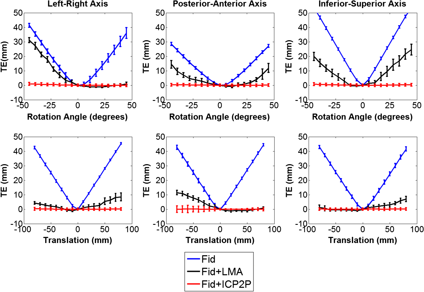

3.2.3.

Effects of the number of digitized locations and extracted scalp points

In order to compare the performances of LMA and ICP2P, it is necessary to use the same initial guess for both. Because LMA typically converges onto largely incorrect solutions ($\mathrm{TE}>50\mathrm{mm}$) when starting from an initial guess based on CoM, here we report the results obtained using fiducial alignment as the starting point. In contrast, due to its stability irrespective of the starting guess, ICP2P provides the same results when either CoM or fiducial alignment is used as the initial guess (see Fig. 6). In this section, we report results about the stability of each algorithm in the presence of a variable number of digitized locations and extracted scalp points.

For the analysis of the effects of the number of digitized locations, we selected random samples of different sizes from the overall data set of digitized points. Figure 8 shows the group mean TEs (and related standard errors) as a function of the number of digitized points used (up to the maximum number of available digitized points) for the LMA and ICP2P algorithms. These results indicate that in actual data, ICP2P and LMA require $\sim 250$ to 300 digitized points in order to provide stable results, after which there are diminished returns when the number of points is increased further. However, ICP2P is more affected by undersampling (higher average TEs). As suggested by the simulations, this may be due to the presence of a small spatial distortion (i.e., correlated noise) in our sampling procedure.

Fig. 8

Group mean TEs and related standard errors as function of number of digitized points. Fid + LMA = fiducial alignment followed by LMA, Fid + ICP2P = fiducial alignment followed by ICP2P.

The representation of the scalp surface may also affect the stability of the algorithms. Figure 9 reports the group mean TEs and their standard errors for the LMA and ICP2P algorithms as a function of the number of scalp points representing the surface. This figure suggests that both procedures reach stable results when $>100$ points are used to describe the scalp surface, although ICP2P is more sensitive to scalp undersampling. This is probably because accurate depiction of the scalp curvature requires additional points.

Fig. 9

Group mean TEs and related standard errors as function of number of extracted scalp points (semilogarithmic scale). Fid + LMA = fiducial alignment followed by LMA, Fid + ICP2P = fiducial alignment followed by ICP2P.

3.3.

Effects of Co-Registration Accuracy in Simulated HD-DOT Data

We tested the effect of the amount of co-registration error on HD-DOT data. A 1-cm 10%-increase absorption change was simulated in the primary visual cortex. Figure 10 shows the reconstructed absorption changes for different co-registration errors, overlaid on the anatomical image of one representative subject. The absorption changes are reported in different colors as a function of optode displacement (blue: $\mathrm{TF}=0\mathrm{mm}$, green: $\mathrm{TF}=3\mathrm{mm}$, red: $\mathrm{TF}=9\mathrm{mm}$). For each TF level, the colored area represents the voxels for which the 3-D reconstruction method indicates the presence of a signal of at least 50% of the peak value. When no displacement is introduced (0 mm), the reconstructed absorption change is located in the primary visual cortex and its dimensions are comparable with the original dimensions [average of full width half maximum (FWHM) $13\mathrm{mm}\pm 1.1\mathrm{mm}$, average displacement (DS) $0.8\mathrm{mm}\pm 0.4\mathrm{mm}$]. When a small TF is introduced (3 mm), similar results are obtained (no statistical difference on group analysis: average FWHM $15\mathrm{mm}\pm 1.3\mathrm{mm}$, DS $1.2\mathrm{mm}\pm 0.2\mathrm{mm}$, $t(4)=1.2$, n.s.). When a bigger TF is introduced (9 mm), the reconstructed absorption change is shifted by a significant amount and appears to be more superficial, with bigger FWHM and higher levels of noise (group analysis: FWHM $29\mathrm{mm}\pm 2.2\mathrm{mm}$, DS $18.2\mathrm{mm}\pm 2.2\mathrm{mm}$; TF 9 mm versus TF 0 mm, FWHM $t(4)=4.2$, $p<0.01$, DS $t(4)=6.6$, $p<0.01$).

Fig. 10

Reconstructed primary visual cortex absorption changes plotted on the MRI of one representative subject. Different colors represent different optodes displacement (translational factors) between the forward and inverse solutions. Absorption changes are displayed up to an attenuation of 50%.

4.

Discussion

For all functional brain imaging techniques that do not provide anatomical information directly, accurate, stable, and fast procedures are required for co-registering digitized sensor locations to their correct anatomical locations. An automatic algorithm stream is desirable in order to avoid time-consuming approaches and errors.

In this paper, we considered two (nonmutually exclusive) approaches: fiducial alignment and surface fitting. Fiducial alignment is simple and relatively fast. However, in our study, its accuracy was limited (errors are $\sim 9\mathrm{mm}$ on average). Further, it is very sensitive to human errors, which can easily occur as it is largely based on manual placement of the fiducial markers. Surface-fitting algorithms can be more accurate than fiducial alignment (errors can be $<3\mathrm{mm}$ on average, depending on the procedure used). However, they require a large number of digitized points (250 to 300) spread evenly over the head surface, an accurate scalp extraction algorithm, and an accurate initial guess.

Whalen et al.²³ showed that fiducial alignment followed by LMA outperformed fiducial alignment alone when co-registering the digitized points to the extracted head surface. However, LMA requires a relatively accurate initial guess and, therefore, needs to be coupled with fiducial alignment. The data indicate that the coupling of initial guess estimation based on fiducial alignment and the application of LMA for surface fitting produce reliable results. The accuracy of the fitting, however, still largely relies on the accuracy of the initial guess—with unstable results if the initial guess is incorrect. In addition, this procedure requires manual placement of fiducial markers during the digitization and the anatomical MR recording sessions, as well as manual tracing of the markers from the MR image. Both of these steps are time-consuming and require expertise.

In this paper, we introduced an alternative surface-fitting method never used before for scalp recording co-registration, ICP2P. This method differs from LMA (and other previously proposed surface-fitting methods^21–24) in that it is not only based on the minimization of the distances between points on the two surfaces to be fit (the surface formed by the digitized points and that of the scalp obtained from an MR image), but also relies on normals to the destination surface. Because of this, the point-to-plane minimization method emphasizes regions of high curvature. This is useful because there are very few areas with high curvature on the surface of the scalp (which is generally locally smooth). The paucity of these points may help to reduce ambiguity in the results of the fitting algorithm and facilitates the search for a true minimum. For this reason, we expected this algorithm to generate stable results even in the presence of large errors in the initial guess.

We evaluated the methods using both simulated and actual data from the Whalen et al.²³ study. Simulations indicate that ICP2P is, in fact, less sensitive to initial guess displacement when compared to LMA and is also less affected by low spatial sampling density when just Gaussian noise is present. However, ICP2P appears to be more sensitive to low spatial sampling density than LMA when spatially correlated noise is present at the digitized locations. This requires a high sampling rate to reach a good level of accuracy for all noise conditions. Real scalp digitizations frequently have some amount of correlated noise in the data, and this needs to be taken in consideration. Based on the simulation results (Fig. 5), if the average noise of the digitization process is not too high ($\sim 3\mathrm{mm}$), a spatial sampling of 1 to 2 cm (for a total of 250 to 300 points digitized) is needed to get optimal co-registration accuracy. Real data indicated that the different fitting procedures had equivalent overall accuracy (provided that scalp curvature correction was used). Note, however, that in order to reach this level of accuracy with LMA, it is necessary to use fiducials to generate the initial guess. Instead, the ICP2P algorithm reached this level of accuracy when either the fiducial method or the CoM method (a completely automatic method not requiring additional action by the experimenter) was used to generate the initial guess.

We also tested the performance stability of both LMA and ICP2P on real scalp-sampled points, as a function of variations in rigid rotation and in the initial guess (based on fiducial alignment). In agreement with simulation results, both iterative procedures yielded small errors when the initial guess was slightly manipulated, but only ICP2P was able to produce robust results even when large rotations and translations were added to the initial guess. These results support the hypothesis that ICP2P provides robust co-registration, which is largely independent of the way in which initial guesses are made. This insensitivity to the initial guessing problem makes it possible to use an entirely automated co-registration method, such as the one using the CoM, for generating the initial guess, followed by ICP2P for surface fitting—which may be very convenient in practical applications.

This advantage was mitigated by the observation that for real data (as well as simulated data with correlated noise) ICP2P is more affected by low density sampling. This probably reflects the fact that real data often contain correlated noise.

The ICP2P procedure was also sensitive to the level of detail used to describe the scalp surface. Since ICP2P relies on estimated normals and curvatures of the destination surface, the need of more scalp points is not surprising. However, most structural MR images provide sufficient detail ($>1000$ scalp points) to generate good co-registration results.

The ICP2P method also benefitted from a procedure called curvature correction, in which curvature outliers were eliminated from the data. Since this procedure is entirely automatic, it can be implemented in the software in a manner that does not require operator intervention, and it, therefore, does not introduce any practical difficulties. In this study, this was a critical step due to the presence of the donut-shaped markers on the scalp during MRI scanning.

It should be noted that the co-registration algorithms appear to reach an asymptotic level of accuracy of $\sim 3\mathrm{mm}$. This level of accuracy depends on a number of factors that are inherent to the methods used for co-registration. They include the spatial sampling of the anatomical MRI ($\sim 1\mathrm{mm}$), the error provided by the 3-D digitizer (estimated at $\sim 0.8\mathrm{mm}$), the placement error of the digitizing instrument and of markers (possibly $\sim 1$ to 2 mm for skilled operators), and various further errors introduced by spatial filtering, rotations, and so on (possibly $\sim 1$ to 2 mm). If we assume that all these errors are independent of each other, their total effect should be equivalent to the square root of the sum of the squared errors. This, in fact, corresponds closely to the best observed TE, suggesting that the proposed methods are very close to reaching the upper limit in terms of possible co-registration accuracy and that any further improvement is not likely to come from a better co-registration algorithm per se but rather from smaller errors in each of the steps contributing to the data used for the co-registration (i.e., the co-registration problem is data-limited rather than algorithm-limited).

For the surface-based recording modalities for which these co-registration methods are likely to be used (such as diffuse optical imaging and EEG), the error introduced by co-registration is smaller than the level of spatial resolution that can be expected from the technique (at least with current methods). Therefore, in none of these cases does the co-registration error represent the main limiting factor in the accuracy of the spatial representation of the data. It should be noted, however, that this is not necessarily the case for the simplest co-registration method based on the use of fiducial points alone. In this case, the error of co-registration may be comparable with, or even larger than, the possible spatial resolution of the technique and, therefore, could be an important contributor to errors in the accurate spatial representation of the data.

To this end, we tested the effects of the amount of co-registration error on simulated 3-D reconstructed HD-DOT data. The results indicate that when a small error is introduced (3 mm, comparable with the errors obtained with surface-fitting procedures), the 3-D reconstruction is not significantly affected by the co-registration error. However, when a bigger error is introduced (9 mm, comparable with fiducial alignment errors), 3-D reconstruction shows large errors (bigger than the optode displacement errors) in both the localization of the inhomogeneity and its dimensions. In other words, when the co-registration error is close to the intrinsic spatial resolution of the method (point spread function $\sim 1.3\mathrm{cm}$; Ref. 13), it is likely to lead to errors in the estimation of the location of the optical signals.

5.

Conclusions

Functional brain imaging techniques that rely on scalp recording sensors require accurate and stable co-registration algorithms for correct alignment to anatomical locations. An automatic algorithm is desirable in order to avoid human errors and time-consuming procedures. We considered two (nonmutually exclusive) algorithms: fiducial alignment and iterative surface-fitting procedures. Fiducial alignment is simple, but it is not automatic and has low accuracy ($\text{average errors}=9\mathrm{mm}$). Surface-fitting algorithms (LMA and ICP2P) are more accurate ($\text{average errors}=3\mathrm{mm}$). However, they rely on iterative procedures, which require accurate scalp representations, an initial guess, and a dense and uniform sampling of the head surface (250 to 300 digitized points). There were trade-offs between LMA and ICP2P: compared to LMA, ICP2P was less robust to correlated noise and sampling strategies, but less sensitive to the accuracy of the initial guess, to the point that it could be based on a completely automated procedure. Considering the intrinsic spatial resolution of HD-DOT data, surface-fitting algorithms may be particularly useful to reduce co-registration errors.