Localizing fluorophore (centroid) inside a scattering medium by depth perturbation

Tuo Zhou; Takehiro Ando; Keiichi Nakagawa; Hongen Liao; Etsuko Kobayashi; Ichiro Sakuma

doi:10.1117/1.JBO.20.1.017003

22 January 2015 Localizing fluorophore (centroid) inside a scattering medium by depth perturbation

Tuo Zhou, Takehiro Ando, Keiichi Nakagawa, Hongen Liao, Etsuko Kobayashi, Ichiro Sakuma

Author Affiliations +

Journal of Biomedical Optics, Vol. 20, Issue 1, 017003 (January 2015). https://doi.org/10.1117/1.JBO.20.1.017003

Abstract

Fluorescence molecular tomography (FMT) imaging can be used to determine the location, size, and biodistribution of fluorophore biomarkers inside tissues. Yet when using FMT in the reflectance geometry it is challenging to accurately localize fluorophores. A depth perturbation method is proposed to determine the centroid of fluorophore inside a tissue-like medium. Through superposition of a known thin optical phantom onto the medium surface, the fluorophore depth is deliberately perturbed and signal localization is improved in a stable way. We hypothesize that the fluorophore centroid can be better localized through use of this fluorescent intensity variation resulting from the depth perturbation. This hypothesis was tested in tissue-like phantoms. The results show that a small-size fluorophore inclusion (1.2 mm³ volume, depth up to 4.8 mm) can be localized by the method with an error of 0.2 to 0.3 mm. The method is also proven to be capable of handling multiple fluorescent inclusion conditions with the assistance of other strategies. Additionally, our further studies showed that the method’s performance in the presence of background fluorophores indicated that the small inclusion could be located at a 1.8 (3.8) mm depth with accurate localization only when its concentration was not <10 (100) times the background level.

1. Introduction

The emergence of fluorescent imaging enables noninvasive, repetitive, and real-time observation of living cells, tissue samples, organs, and even the entire bodies of small animals. It always works with fluorophore-loaded imaging agents that ideally only accumulate in diseased tissues. Thus it provides contrast for imaging disease foci. Clinically, this technique has been already used for tumor diagnosis,¹ surgery margin,²^,³ and the removal of residual tumors.⁴ In preclinical applications, owing to its low-cost nature, fluorescent imaging serves as a tool for evaluating molecular imaging agents before the agents are tested on other expensive modalities, such as magnetic resonance imaging.⁵ The primary limitation of fluorescent imaging arises from the high scattering and absorption of photons in biological tissue, which leads to a blurred fluorescent profile on the tissue surface. Hence, the accurate determination of the size and location of fluorophore-loaded imaging agents (i.e., diseased tissues) becomes difficult.⁶

Consequently, various types of fluorescence molecular tomography (FMT) have been developed to determine the depth, size, and three-dimensional (3-D) distribution of fluorophores inside tissues from blurred fluorescent signals on the tissue surface.⁷^,⁸ Among them, FMT that uses a circular geometry where detectors and sources are positioned as surrounding the subject,⁹^,¹⁰ is the most common type. However, owing to the limited optical penetration depth, applications of this type are mainly limited to small animals or ex vivo samples. As an alternative, FMT with reflectance geometry,¹¹^–¹⁴ where the light source and detector are placed on the same side, shows greater promise for usage in clinical fields. First, it is suitable for imaging exterior organs (such as skin, mouth, and so on), and second, during brain and thoracic surgeries, a reflectance geometry system can work without obstruction from the skull and chest, thus extending the penetration depth. Because all detectors and sources are placed on the same side that is observed by the doctor, only a few additional operations are required to set them up.

Like any tomography technique, resolving depth is an extremely crucial issue in the field of FMT. In the circular geometry, depth information can be extracted from intensity difference among detectors. For instance, the fluorophore is very probably closer to a side with stronger signals. However, in the reflectance geometry, this is not feasible because all the detectors and sources are placed on the same side. As alternatives, two strategies have already been reported. One is called source-detector separation,¹¹^–¹³^,¹⁵ which assumes different source-detector distances can provide depth information. It always involves with inversion of a sensitivity matrix relating the source-detector positions to the fluorophore distribution. The matrix usually has a large scale and is ill-conditioned, i.e., extremely sensitive to noise.¹⁶ The sensitivity to noise is important because fluorescent signals in the reflectance geometry are noisier than those in other geometries because of the existence of autofluorescence and excitation light leakage.⁶ The other method is multispectral fluorescence imaging. This method relies on the fact that tissue optical attenuation varies with the light wavelength. This strategy was first proposed by Swartling et al.¹⁷^,¹⁸ and was recently analytically described by Leblond et al.¹⁹ We positively evaluated the effect of this study but noticed that its feasibility is restricted in the wavelength band where tissue optical properties drastically change with light wavelength. However, the dependency of optical coefficients on wavelength is actually extremely complicated. In some wavelength bands, scattering decreases with wavelength, while absorption increases with an increasing wavelength. Therefore, the effective optical attenuation may not significantly change. On the other hand, in multispectral fluorescence imaging, fluorescence is independently measured at several isolated bands (the bandwidth is 10 nm in Ref. 19) of different wavelengths. The fluorescent strength over a narrow band is apparently much weaker than that of the integrated fluorescence. Therefore, low detecting sensitivity is another issue of the method.

For accurately resolving fluorophore depth in more general conditions, we previously proposed a depth perturbation method.²⁰ A thin optical phantom with known optical properties is used as a depth perturbator. By superposing the perturbator onto a sample, we deliberately perturb the depth of the fluorophore inside the sample. Fluorescent signals are measured before and after perturbation. According to variations in the measurements, depth information can be obtained. Herein, we hypothesize that not only fluorophore depth, but also its location can be determined by the depth perturbation. For a fluorophore of finite size, the determined location will appear around its centroid because of averaging. Knowing the centroid, researchers can use a spatially varying regularization method²¹^–²³ to mitigate the ill condition of the optical inverse problem and to more accurately reconstruct fluorophore distribution. We tested the hypothesis with tissue-like phantoms and a mesoscopic epifluorescence tomography (MEFT). MEFT can detect fluorophore distribution in reflectance geometry at depths of several millimeters.¹³ Owing to its limited detection depth and field of view, we mainly focus on detecting small-size fluorophores ( $diameter = 0$ to 2 mm). Here we focus on describing the principles, procedures, and performance evaluation of the depth perturbation method. For details on the reconstruction method with a centroid prior, see Ref. 24.

2. Method

2.1.

Depth Perturbation

The concept of depth perturbation emerged from the diffusion equation of photon transport in a scattering medium.²⁵ First, consider the situation shown in Fig. 1(a). A pencil laser beam is normally incident on a semi-infinite scattering medium. If the refractive index mismatch at the air-medium boundary is ignored, the fluence rate of excitation light at the point O, i.e., a location $d$ beneath the incident point, can be expressed as

Eq. (1)

φ_{ex}^{0} (d) = C_{ex} \exp (- μ_{eff}^{ex} d^{'}) / d^{'},

where

μ_{eff}^{ex} = \sqrt{3 μ_{a, ex} (μ_{a, ex} + μ_{s, ex}^{'})}

denotes the effective attenuation coefficient at the excitation wavelength (

μ_{a, ex}

and

μ_{s, ex}^{'}

are absorption and reduced scattering coefficients at the excitation wavelength, respectively);

C_{ex} = α^{'} P / (4 π D_{ex})

is a constant consisting of incident power

P

, light diffusion coefficient

D_{ex} = 1 / (3 μ_{a, ex} + 3 μ_{s, ex}^{'})

, and albedo

α^{'} = μ_{s, ex}^{'} / (μ_{a, ex} + μ_{s, ex}^{'})

; and

d^{'} = d - l_{t}^{'}

is the distance from the virtual excitation source S (approximation of the pencil beam) to O, where

l_{t}^{'} = 1 / (μ_{a, ex} + μ_{s, ex}^{'})

. Then, assuming a fluorescent point source at O and continuing to ignore the refractive index mismatch, the emission fluence rate at point A can be solved as

Eq. (2)

φ_{em}^{0} (d) = C_{em} \exp (- μ_{eff}^{em} d) / d,

where

μ_{eff}^{em} = \sqrt{3 μ_{a} (μ_{a, em} + μ_{s, em}^{'})}

denotes the effective attenuation coefficient at the emission wavelength whose absorption and reduced scattering coefficients are

μ_{a, em}

and

μ_{s, em}^{'}

, respectively;

C_{em} = c κ η / (4 π D_{em})

is another constant consisting of fluorophore amount

c

, extinction coefficient

κ

, and quantum yield

η

as well as a diffusion coefficient at emission wavelength

D_{em} = 1 / (3 μ_{a, em} + 3 μ_{s, em}^{'})

. Therefore, fluorescence intensity at point A is

Eq. (3)

Φ_{0} = φ_{ex}^{0} (d) φ_{em}^{0} (d) .

Fig. 1

Schematic of depth perturbation: (a) initial status [two-dimensional (2-D)], (b) after perturbation (2-D), (c) initial status [three-dimensional (3-D)], (d) after perturbation (3-D). Circles denote observation points, and triangles denote virtual point sources corresponding to the laser beams.

Finally, a perturbator of thickness $Δ d$ is superposed onto the medium [Fig. 1(b)]. For simplicity, optical properties of the perturbator are assumed to be same as those of the medium. The fluorescence intensity at A can, thus, be expressed as

Eq. (4)

Φ_{1} = φ_{ex}^{0} (d + Δ d) φ_{em}^{0} (d + Δ d) .

Consequently, at A, the ratio of fluorescence intensity after the perturbation to that before can be calculated as

Eq. (5)

Γ = \frac{Φ_{1}}{Φ_{0}} = \exp [- (μ_{eff}^{ex} + μ_{eff}^{em}) Δ d] \frac{d - l_{t}^{'}}{d - l_{t}^{'} + Δ d} \frac{d}{d + Δ d},

where constants

C_{em}

and

C_{ex}

(as well as other factors like the sensitivity of the measuring system) were canceled out. Although being analytically complex,

Γ

is actually a monotonic increasing function of

d

as shown in Fig. 2. Light attenuation within the medium is affected by the light effective propagation distance. For the condition shown in Figs. 1(a) and 1(b), the depth perturbation prolongs the effective propagation distance of either the incident excitation light or the emitted fluorescence from

d

to

d + Δ d

. This, thus, results in the decrease of excitation light fluence rate at point O (fluorophore position), and also the decrease of the fluorescence fluence rate at point A (observing point). The key point is, the larger

d

is, the smaller

Δ d / d

(the relative variation of the distance) will be. That is, the relative decreases of the excitation light fluence rate, emission fluence rate, and, thus, fluorescence intensity at A are smaller for a larger

d

. As a result, the intensity ratio

Γ

increases with

d

, i.e., fluorophore depth. On the basis of this dependency of

Γ

on the fluorophore depth, we can in turn obtain depth information by observing the intensity variation owing to the perturbation.

Fig. 2

Intensity ratio owing to the perturbation versus fluorophore depth: the ratio is calculated from Eq. (5) using the optical coefficients and perturbator thickness similar to those of the phantom experiments (described later).

2.2.

Extension to 3-D Volume

Because Eq. (5) is valid only when both the incident point (position vector $r_{s}$ ) and observation point $r_{d}$ are just above the fluorophore $r_{f}$ , and because the horizontal position of the fluorophore may be unknown, we practically generalized Eq. (1) $\sim 5$ from the extreme condition shown in Figs. 1(a) and 1(b) to any given excitation source point or observation point [Figs. 1(c) and 1(d)] in a 3-D volume, by replacing $d^{'}$ in Eq. (1) with $| r_{s} - r_{f} |$ , $d$ in Eq. (2) with $| r_{d} - r_{f} |$ , and some other modifications. Therefore, $Γ$ actually depends on perturbator thickness $Δ d$ and relative positions among detection point $r_{d}$ , incident point $r_{s}$ , and fluorophore $r_{f}$ . This dependency can be forward modeled on the basis of either the diffusion equation or Monte Carlo simulation.²⁶

In the forward process, a fluorescent object of finite size is approximated as a point source at the object centroid. This approximation is valid since, in this study, we focus on localizing fluorophores of small size. Unlike ignoring the boundary condition and the optical mismatch in the last section, here, to consider factors such as boundary condition, optical mismatch between the perturbator and medium, laser beam size, and so on, we used numerical simulations based on the diffusion equation and the finite element method²⁷ to calculate the theoretical fluorescent intensity before the perturbation $Φ_{0}$ and that after the perturbation $Φ_{1}$ for any given $r_{s}$ , $r_{d}$ , $r_{f}$ , and $Δ d$ . If there is only one fluorescent object inside the medium, the forward model can be expressed as

Eq. (6)

Γ (r_{s}, r_{d}, r_{f}, Δ d) = \frac{Φ_{1} (r_{s}, r_{d}, r_{f}, Δ d)}{Φ_{0} (r_{s}, r_{d}, r_{f})} .

If there are multiple objects simultaneously in the examined region, $Γ$ can be calculated as

Eq. (7)

Γ (r_{s}, r_{d}, m, Δ d) = \frac{\sum_{i = 1}^{n} c_{i} Φ_{1} (r_{s}, r_{d}, r_{f}^{i}, Δ d)}{\sum_{i = 1}^{n} c_{i} Φ_{0} (r_{s}, r_{d}, r_{f}^{i})},

where

m = (c_{1}, r_{f}^{1}, \dots c_{i}, r_{f}^{i} \dots c_{n}, r_{f}^{n})

;

c_{i}

and

r_{f}^{i} = (x_{i}, y_{i}, z_{i})

denote the amount of fluorescent molecules (fluorophore molar concentration × object volume) and position vector of the

i

’th object, respectively; and

n

denotes the number of objects inside the medium. The denominator (numerator) of this equation is the total fluorescence intensities integrating the contributions of all fluorophore objects before (after) the perturbation. Representative distributions of

Γ

were shown in Fig. 3. One can note that the ratio increases with an increasing distance from the observation point to the fluorophore [Fig. 3(a)]. Similarly, when the incident point moves away from the fluorophore [Fig. 3(b)] or when the fluorophore locates more deeply [Fig. 3(c)], ratios over the image notably increase. These are attributable to the fact that the longer the initial effective propagation distance (incident point → fluorophore → observation), the less is the relative variation of the distance resulting from a given perturbation.

Fig. 3

Representative distributions of $Γ (r_{s}, r_{d}, m, Δ d)$ : (a) the distribution when the laser incident position is horizontally close to a fluorescent point source; (b) the one when the incident position is moved far from the source; (c) the one when the point source is more deeply fixed. On each subfigures, the • denotes horizontal position of the fluorescent point source and its initial depth $d$ is shown in titles. × denotes the laser incident point. Each pixel in the figure represents an observation point. Optical coefficients and perturbator thickness similar to those of the phantom experiments (described later) are used here. The three subfigures share the same color bar.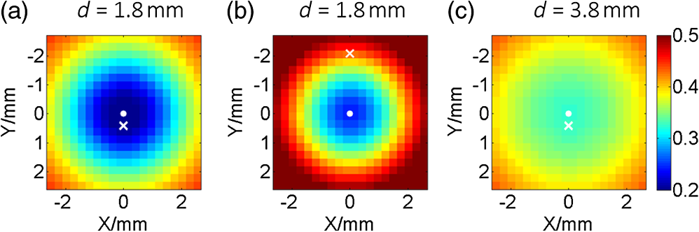

2.3.

Inverse Process

In the inverse process, the measured ratio is calculated as

Eq. (8)

R (r_{s}, r_{d}, Δ d) = I_{1} (r_{s}, r_{d}, Δ d) / I_{0} (r_{s}, r_{d}),

where

I_{0}

and

I_{1}

are fluorescent images before and after the perturbation. Then, the fluorophore location(s), as well as relative fluorescent amount(s), can be estimated by fitting the measured intensity ratios

R

to the forward model

Γ

, using the expression as follows:

Eq. (9)

\min {‖ [\begin{matrix} R (r_{s}^{1}, r_{d}^{1}, Δ d) \\ R (r_{s}^{1}, r_{d}^{2}, Δ d) \\ ⋮ \\ R (r_{s}^{i}, r_{d}^{j}, Δ d) \\ ⋮ \\ R (r_{s}^{N_{s}}, r_{d}^{N_{d}}, Δ d) \end{matrix}] - [\begin{matrix} Γ (r_{s}^{1}, r_{d}^{1}, m, Δ d) \\ Γ (r_{s}^{1}, r_{d}^{2}, m, Δ d) \\ ⋮ \\ Γ (r_{s}^{i}, r_{d}^{j}, m, Δ d) \\ ⋮ \\ Γ (r_{s}^{N_{s}}, r_{d}^{N_{d}}, m, Δ d) \end{matrix}] ‖}_{2},

where

N_{s}

and

N_{d}

are the number of sources and detectors, respectively;

r_{s}^{i}

and

r_{d}^{j}

denote the

i

’th source position and the

j

’th observation position, respectively. We utilized nonlinear regression [Levenberg-Marquardt (LM) method] for the fitting and a multistart strategy to circumvent the LM method from converging to a local minimum. For details of the LM method and the multistart strategy, see Ref. 16.

2.4.

Deciding Fluorophore Number

For more generality, we took a “try from one” strategy to handle the condition that the number of fluorescent objects inside the examined region is unknown. We first assumed the number as $n$ ranging from 1 to $N$ (i.e., $N = 5$ ); second, we ran the nonlinear regression for each $n$ ; third, we substituted the solution $m_{n}$ back to the theoretical ratio model $Γ (m)$ to calculate the residuals as $Res (n) = {‖ Γ {(m}_{n}) - R ‖}_{2}$ . We noticed that when the assumed number $n$ is smaller than the true value, the residual is large; in contrast, if $n$ is equal to or more than the true value, it decreases to a relatively lower and stable level. For an underestimated $n$ , parameters used in the regression are too few to achieve good fitting results; for an overestimated $n$ , the overestimated object(s) usually appear as object(s) of extremely small amounts or those present at a large depth; i.e., they merely contribute to the fitting result. By detecting the turning point on $Res (n)$ , we can decide the object number. The turning point is defined as the first $n$ (from 1 to $N$ ) whose residual variation rate,

Eq. (10)

rate (n) = \frac{| Res (n) - Res (n + 1) |}{Res (n)},

is less than a threshold

ε

. Herein we empirically selected the threshold as

ε = [1.2 \sum_{1}^{N} rate (n)] / N

[i.e., 1.2 times the mean value of rate (

n

) over

n = 1

to

N

]. After this try from one strategy, we also set other limits to eliminate some obviously incorrect estimates. For instance, an object at a very large depth (

> 10 mm

) was ignored; two estimated objects located extremely close to each other (distance

\leq 0.1 mm

) were counted as one object.

2.5.

Preliminary Study on the Effects of Background Fluorescence

Finally, the performance of the proposed methods in the presence of background fluorescence was preliminarily studied. Herein, background fluorescence refers to fluorescence not emitted from the fluorescent object that we are attempting to localize. Reasons for background fluorescence include endogenous fluorophore (autofluorescence) or the distribution of exogenous fluorescent dyes outside the targeted tissue.²⁸ (Although fluorescent dyes are supposed to accumulate in the targeted tissue, owing to the imperfect current fluorescent imaging agents, they are more or less residual in the background tissue.) With the presence of background fluorescence, raw measured fluorescent images before the perturbation (after the perturbation) can be expressed as $I_{0} = I_{0}^{tar} + I_{0}^{back}$ ( $I_{1} = I_{1}^{tar} + I_{1}^{back}$ ), where $I_{0}^{tar}$ ( $I_{1}^{tar}$ ) denotes intensity contributions from the fluorescent object before (after) the perturbation, and $I_{0}^{back}$ ( $I_{1}^{back}$ ) denotes intensity contributions from background fluorophores before (after) the perturbation. As a result, the raw intensity ratios $I_{1} / I_{0}$ may significantly differ from the target intensity ratio $I_{1}^{tar} / I_{0}^{tar}$ . When applying $I_{1} / I_{0}$ to the inverse process, one obtains the weighted centroid of fluorophores over the entire tissue. But, to localize the fluorophore target, we first have to remove the background fluorescence component.

As a preliminary evaluation, herein we only considered the condition that the background concentration is homogeneous within the tissue of interest. In this case, to obtain background fluorescence images, we can simply transfer the laser beam to an incident position distant (i.e., 10 mm away) from the fluorophore object (the rough horizontal location of a fluorescent object can be determined by coarsely scanning the laser beam over the sample and comparing the brightnesses of images captured at all incident positions), and assume that the image captured in this condition included background fluorescence only. Then, after spatial registration and data interpolation, the background fluorescence components were subtracted from the raw fluorescent images (captured under the usual beam scan) to obtain the target fluorescence components. A similar method was previously used in Ref. 29, where the effect of background fluorescence on transmission geometry FMT was investigated.

3. Experiments and Materials

The proposed methods and procedures were tested by tissue-like phantoms and an MEFT system.

3.1.

Phantom

In the phantom, a mixture of intralipid, ink, and water was used to mimic scattering and absorption properties of biological tissues. Optical coefficients of the mixture are close to those of the brain cortex:³⁰ reduced scattering coefficient $μ_{s, ex}^{'} = 11.7 {cm}^{- 1}$ , absorption coefficient $μ_{a, ex} = 0.2 {cm}^{- 1}$ at excitation wavelength 785 nm; $μ_{s, em}^{'} = 10.5 {cm}^{- 1}$ , $μ_{a, em}^{'} = 0.2 {cm}^{- 1}$ at the emission peak wavelength 830 nm of indocyanine green (ICG, the fluorophore used herein, absorption maximum 780 nm, emission maximum 830 nm,³¹ Keisei, Japan). A fixed volume of ICG solution, diluted with the mixture, was injected in a capillary tube (inner diameter: $Φ$ 1.0 mm) to make an isolated ICG object. The object length is $\sim 1.5 mm$ . All ICG objects used in this study are nearly of the same size.

We conducted experiments with three phantom configurations:

C1: One ICG object was submerged and fixed inside a plastic tank ( $40 \times 90 \times 50 {mm}^{3}$ ), which was filled by the tissue-like mixture. By adjusting the volume of the mixture inside the tank, the initial central depth of the tube was changed from 1.8 to 4.8 mm in 1-mm intervals. The concentration of this ICG object was $1 μ M$ . No background fluorophore was added into the phantom [see Figs. 4(a) and 4(b)].

Fig. 4

Schematic of the phantoms. (a) Schematic of phantom configuration C1: one tube, no background fluorescence, and liquid perturbator (not shown). (b) The $Y - Z$ cross-section of (a). (c) Schematic of phantom configuration C2: two tubes at different depths, no background fluorescence, and liquid perturbator (not shown). (d) The $Y - Z$ cross-section of (c). (e) Schematic of phantom configuration C3: one tube, $0.01 μ M$ indocyanine green background fluorescence, and solid perturbator. (f) The $Y - Z$ cross-section of (e).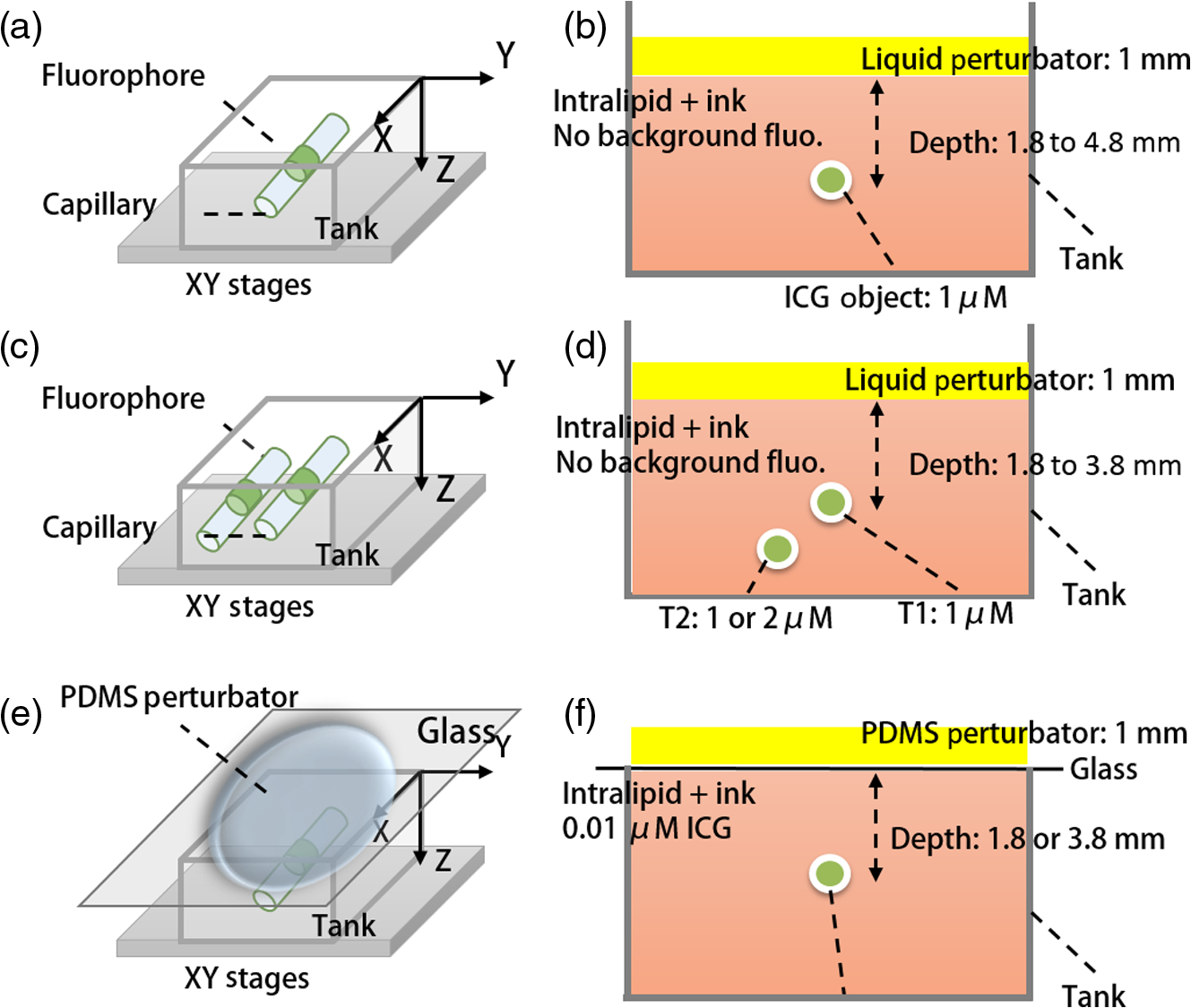

C2: Two tubes, T1 and T2, were immersed into the mixture. The ICG concentration in tube T1 was fixed at $1 μ M$ , whereas that of T2 was $2 μ M$ , $1 μ M$ sequentially. Thus, the ratio of fluorophore amount $c_{T 2} / c_{T 1}$ was set to 2 and 1, respectively. The initial depth of T1 varied from 1.8 to 3.8 mm, whereas T2 was 1 mm deeper than T1 in the vertical direction. Horizontally, T1 and T2 were separated by 1 mm (edge-to-edge) along the $Y$ direction and centered at nearly the same coordinate along the $X$ direction. No background fluorophore was added into the phantom [see Figs. 4(c) and 4(d)].

C3: Configuration C3 was modified from C1 (one tube, tube central depth: 1.8 or 3.8 mm) by the further addition of $0.01 μ M$ ICG background fluorophore. We sequentially set the ICG concentration inside the tube as 10, 1, and $0.1 μ M$ . The target to background concentration ratio $c_{T} / c_{B}$ was 1000, 100, and 10, respectively. A blank phantom test (devoid of fluorescent object) was also performed on this configuration [see Figs. 4(e) and 4(f)].

The objectives of the experiments on these three phantom experiments were different. Experiments on C1 were used to verify the proposed method’s ability to localize fluorophore centroids. Experiments on C2 were performed to investigate whether the proposed method can handle the multiple-objects cases. These two are proof-of-concept configurations. For C3, the experiment was implemented in more realistic conditions to establish the sensitivity limit of the proposed method under the current MEFT system.

3.2.

Perturbator

On the basis of the configuration objective, different perturbators were used in their respective experiments. For the proof-of-concept configurations, C1 and C2, we used the same tissue-like mixture with a 1 mm fixed thickness as the depth perturbator for convenience and computational simplicity. For C3, to more realistically simulate practical applications, we used a solid perturbator that has optical properties different from the background mixture [Fig. 4(e)]. The solid perturbator was a piece of membrane made of polydimethylsiloxane (PDMS). As a widely used silicon-based organic polymer, PDMS is optically clear, nontoxic, and flexible.³² Therefore, a perturbator made of PDMS could be tightly attached to biological tissues even on a nonplanar irregular surface. By mixing ${TiO}_{2}$ (scatter) into PDMS, the reduced scattering coefficient of the perturbator was adjusted to $0.65 {cm}^{- 1}$ (absorption is nearly 0). It had a round shape, diameter of 45.0 mm, and a thickness of 1.0 mm. To support the PDMS perturbator, a very thin glass slide was covered onto the tank, which was filled by the tissue-like mixture [for C1 and C2, the tank was not initially filled for leaving space for the liquid perturbator, see Figs. 4(b), 4(d), and 4(f)]. For the depth perturbation, the PDMS perturbator was superposed on the glass slide. The effect of the glass was considered in the forward process.

3.3.

Measuring System

In the MEFT system (Fig. 5), a fiber pigtailed laser diode (785 nm, LP785-SF20, Thorlabs, USA) was used as the light source. The laser light was collimated to a $460 - μ m$ diameter and 10 mW power Gaussian beam. The X-Y motorized stages allowed the laser beam to scan over a sample in a maximal travel range of 20 mm. Herein, the beam was translated to produce a raster scan of $10 \times 10$ incident points with a step of 0.5 mm. A notch filter, bandpass filter, two polarizing beam splitters (PBS), and a dichroic mirror (DM) rejected ambient light and reflection of excitation light. In particular, the two PBS were used to eliminate the specular reflection of the laser beam. The left PBS transmits the incident beam as a nearly pure S polarization light. The specular reflection of the beam is still S polarized because specular reflection does not change light’s polarization properties. Finally, the right PBS reflects (i.e., rejects) all S polarization content. As a result, the specular reflection was rarely detected by the camera.

Fig. 5

Schematic of the mesoscopic epifluorescence tomography system.

Fluorescence was collected by an electron multiplying charge coupled device (EMCCD) camera (resolution $1000 \times 1000$ , ADT-100, Flovel, Japan). In the EMCCD camera, one photon can be amplified to several thousands of electrons, thus allowing the measurement of a very weak fluorescent signal. The camera was adjusted and calibrated carefully so that the lens plane was parallel to the air-medium surface. The vertical distance from the camera to the sample top surface is 13 cm (upon the height of sample). The effect of this camera-sample height will be discussed later. Light-collecting efficiencies of the system at different observation positions (corresponding to pixels on the camera) were calibrated beforehand using an optical phantom with a known homogeneous background fluorophore distribution (no additional fluorophore inclusion).

3.4.

Data Preprocessing

On each fluorescent image, we assumed a $5.3 \times 5.3 {mm}^{2}$ square region of interest (ROI) including $20 \times 20$ virtual detectors. Each detector was an $8 \times 8$ camera pixel binning. The ROI was determined according to image brightness. The pixel with the maximum brightness was centered in the ROI. The ROI size was empirically decided to reject all pixels with extremely low brightness (e.g., $< 10 %$ of camera dynamic range) to maintain a good signal-to-noise ratio (SNR). Similarly, for source positions, we selected a subgroup from images captured at the $10 \times 10$ incident points. The mean SNR over the ROI (mathematical definition is described in Sec. 4.1) of a selected image should be $> 25 dB$ , because our previous numerical simulations (data not shown) proved that our LM algorithm works very well (centroid localization error $\approx 0.1 mm$ ) when the mean SNR is not $< 25 dB$ . Furthermore, for shortening the computing time, when $> 10$ (an empirical value) images fulfill the SNR criteria, only the 10 images with the highest SNR were applied to the inverse process.

3.5.

True Fluorophore Location in the Image Coordinates

The left top of the camera image and initial height of the medium surface were set as the $X - Y$ and $Z$ origins of the image (camera) coordinates, respectively. To obtain the true coordinates of the fluorophore horizontal location, we temporally removed all optics between the camera and phantom (fluorophore only, no mixture) and took an image for the fixed fluorophore. From the image, actual $X - Y$ coordinates of the fluorophore centroid could be determined with a precision of 0.03 mm. We also used a height gage (precision: 0.01 mm, Mitutoyo, Japan) with a pin to measure the absolute heights of the surface and the tube to calculate the tube’s relative depth from the surface. These true locations were only used for comparison with the estimating results of the inverse process to calculate the localization errors.

3.6.

System Test

We performed a series of phantom experiments to figure out depth-concentration sensitivity and noise performance of the MEFT system. One ICG object and phantom was configured as C1, except that the ICG concentration was varied from 0.1 to $10 μ M$ and its depth was varied from 1.8 to 4.8 mm. For each condition, we allowed the laser beam to scan along the $Y$ direction and to start from the horizontal centroid of the ICG object, stepping in 0.5 mm. The maximum horizontal separation from incident positions to the object was 3 mm. At each incident position, 10 fluorescent images and one background image (no tube) were captured.

3.7.

Validation Experiments

Validation experiments for the proposed methods were conducted by the following steps:

1. Fixing the tube(s) to predefined depth(s);
2. Measuring background signals;
3. Measuring fluorescent signals with beam scan;
4. Depth perturbation: For C1 and C2, adding the mixture into the tank until the tube(s) depth(s) increased by 1 mm; for C3, superposing the PDMS perturbator onto the phantom (the glass slide);
5. Measuring fluorescent signals again;
6. Repeating steps 1 to 4 at each condition $N = 10$ times.

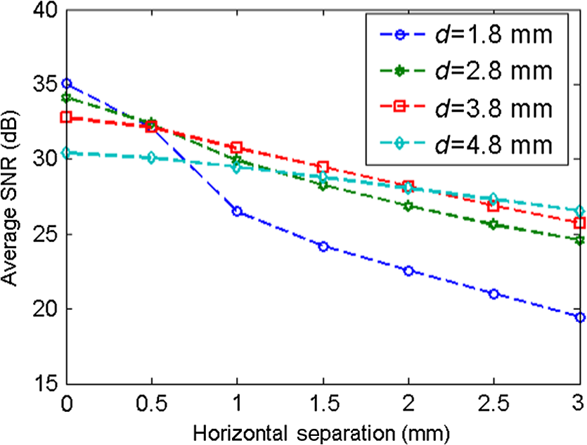
4. Results

Figure 6 shows a group of fluorescent measurements (after pixel binning) where one fluorescent object was set at 3.8 mm depth (configuration C1) and approximately centered on the ROI. The distribution after the perturbation [Fig. 6(b)] was weaker and broader than that before [Fig. 6(a)] because of additional scattering by the perturbator. The intensity ratio map [Fig. 6(c)] shows a similar distribution as the theoretical models (Fig. 3).

Fig. 6

Representative fluorescent measurements (a) before and (b) after the perturbation. (c) Intensity ratio of (b) to (a) • denotes horizontal position of the fluorescent point source and × denotes the laser incident point.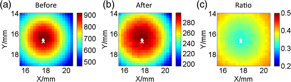

4.1.

System Performance

Two indices were calculated here. One is the detection sensitivity $s$ , which is expressed as $s = \sum_{ROI} I_{a} / T$ , where $\sum_{ROI}$ denotes the brightness summation over the ROI described in Sec. 3.3, $I_{a}$ denotes the image (after background removal and averaging) captured when the incident position was just above the fluorophore centroid, and $T$ is the camera exposure time. Another is the mean SNR (MSNR). SNR at the $i$ ’th pixel on the images was defined as $20 \log_{10} (A_{i} / δ_{i})$ , where $A_{i}$ denotes the average brightness (after background removal) and $δ_{i}$ denotes the standard deviation. MSNR is the average value of the SNR over the ROI.

As shown in Fig. 7, for all four depths, the detecting sensitivity $s$ basically shows good linear dependency on the ICG concentration. The $10 μ M$ data points are always slightly lower than the respective fitted lines, suggesting that the quenching effect may occur at this concentration. Figure 8 shows MSNRs of $1 μ M$ cases, which is the representative concentration used in validation phantom experiments. Data of other concentrations have similar distributions and are omitted for brevity. At this concentration, MSNR was in the range of 20 to 35 dB and decreased with the separation of incident position to fluorophore. This is attributable to the fact that the camera exposure time was set to a fixed value during each beam scan. As a result, signal amplitude, i.e., image brightness, decreased when the incident position moved away from the fluorophore object. This phenomenon is obvious for a small fluorophore depth (e.g., 1.8 mm) because the excitation light does not sufficiently diffuse at this depth.

Fig. 7

System depth-concentration sensitivity.

Fig. 8

System noise performance.

4.2.

Number of Fluorescent Object

In the inverse process, we first estimated the object number $n$ . Figure 9 shows the normalized residuals [ $Res (n) / Res (1)$ , i.e., normalized by the respective value at $n = 1$ ] of C1 and C2 experiments. The residuals among C1 experiments are almost invariant when $n$ was assumed to be 1 to 5 [Fig. 9(a)], whereas among the C2 experiments [Figs. 9(b) and 9(c)], the residuals at $n = 1$ are significantly larger than those at $n \geq 2$ ( $p < 0.01$ ). However, their differences shrink with the fluorophore depth and a decreasing value of $c_{T 2} / c_{T 1}$ . This phenomenon will be discussed in Sec. 5.3. The results of configuration C3 are similar to those of C1 and are not shown here for brevity. Using the strategy and limits described in Sec. 2.4, we correctly identified the object number in all experiments. Solutions of the nonlinear regression corresponding to the decided fluorophore number were selected as the final results. One complete inverse process typically takes 1 to 10 s.

Fig. 9

Relative residual used in the Try From One strategy: normalized relative residual (a) in the C1 configuration ( $tube depth = 2.8$ , 3.8 mm); (b) in the C2 configuration ( $c_{T 2} / c_{T 1} = 2$ , T1 $depth = 2.8$ , 3.8 mm); (c) in the third group ( $c_{T 2} / c_{T 1} = 1$ , T1 $depth = 2.8$ , 3.8 mm). Notice the $Y$ axis scale of (c) is smaller than that of (a) and (b). We do not include other data because most of them overlap on the shown data, thus deteriorating clarity of the figures.

4.3.

Results of C1 Configuration

Table 1 shows the performance of the proposed methods in C1. The localization error $Δ_{tot}$ was defined as the Euclidean distance from the estimated centroid to the actual. $Δ_{Z}$ and $Δ_{Y}$ are the error’s vertical and horizontal components, respectively. For 1.8 to 4.8 mm depths, $Δ_{tot}$ of the proposed method is in the range of 0.20 to 0.30 mm (on average). We also tested a previous method¹³^,³³ based on the source-detector separation (SDS) concept using the same data sets. We first forward modeled the sensitivity matrix of source-detector pairs over the reconstructed space and then reconstructed the fluorophore biodistribution by the LSQR algorithm.³⁴ Finally, the weighted center of the reconstructed distribution was seen as the estimated centroid. For this SDS-based method, its $Δ_{Z}$ increases fast with the fluorophore depth and becomes significantly larger than that of the proposed method ( $p < 0.01$ ), while the $Δ_{X Y}$ of the two methods are similar. [Although averages of $Δ_{X Y}$ of the SDS method are lower, statistically the $Δ_{X Y}$ values of the SDS method are not significantly less than those of the proposed method ( $p > 0.01$ )]. As a result, the total localization errors of the SDS method are also significantly greater than ours ( $p < 0.01$ ). This is attributable to the severe ill-condition of the sensitivity matrix whose condition number is in on the order of $10^{18}$ . These results suggest that the proposed method has better accuracy in resolving depth and localizing the fluorophore centroid.

Table 1

Results for configuration C1 [one tube and no background indocyanine green (ICG)]. All units are in millimeters.

Depth	Depth perturbation			Source-detector separation
Depth	$Δ_{tot}$	$Δ_{Z}$	$Δ_{X Y}$	$Δ_{tot}$	$Δ_{Z}$	$Δ_{X Y}$
1.80	$0.22 \pm 0.07$	$0.20 \pm 0.06$	$0.09 \pm 0.04$	$0.27 \pm 0.03$	$0.26 \pm 0.02$	$0.05 \pm 0.02$
2.80	$0.18 \pm 0.02$	$0.09 \pm 0.01$	$0.16 \pm 0.06$	$0.53 \pm 0.01$	$0.52 \pm 0.01$	$0.07 \pm 0.01$
3.80	$0.28 \pm 0.06$	$0.22 \pm 0.04$	$0.16 \pm 0.08$	$0.71 \pm 0.02$	$0.70 \pm 0.01$	$0.08 \pm 0.01$
4.80	$0.28 \pm 0.04$	$0.24 \pm 0.05$	$0.12 \pm 0.06$	$1.03 \pm 0.01$	$1.02 \pm 0.01$	$0.11 \pm 0.01$

4.4.

Results of C2 Configuration

In the experiments of C2, the localization estimation errors for T1 $Δ_{tot 1}$ and T2 $Δ_{tot 2}$ are listed in Table 2 (the vertical and horizontal components are omitted for brevity). The averages are $\sim 0.3 mm$ and slightly increase with depth. On the other hand, we defined the percentage error of the restored fluorophore amount ratio to the actual as

Eq. (11)

Δ_{c} = 100 % * \frac{| {(c_{T 2} / c_{T 1})}_{est} - {(c_{T 2} / c_{T 1})}_{true} |}{{(c_{T 2} / c_{T 1})}_{true}},

where

{(c_{T 2} / c_{T 1})}_{est}

and

{(c_{T 2} / c_{T 1})}_{true}

denote the restored and true amount ratios, respectively. As listed in Table 2, the percentage errors of

Δ_{c}

are

< 20 %

(on average) for all tested cases.

Table 2

Results for configuration C2 (two tubes and no background ICG).

Depth (mm)	$c_{T 2} / c_{T 1} = 2$			$c_{T 2} / c_{T 1} = 1$
Depth (mm)	$Δ_{tot 1}$ (mm)	$Δ_{tot 2}$ (mm)	$Δ_{c}$ (%)	$Δ_{tot 1}$ (mm)	$Δ_{tot 2}$ (mm)	$Δ_{c}$ (%)
1.8	$0.20 \pm 0.02$	$0.18 \pm 0.02$	$9 \pm 7$	$0.18 \pm 0.02$	$0.19 \pm 0.02$	$7 \pm 6$
2.8	$0.20 \pm 0.04$	$0.21 \pm 0.04$	$18 \pm 12$	$0.20 \pm 0.03$	$0.24 \pm 0.06$	$16 \pm 12$
3.8	$0.23 \pm 0.06$	$0.27 \pm 0.08$	$18 \pm 11$	$0.24 \pm 0.05$	$0.32 \pm 0.09$	$13 \pm 9$

4.5.

Results of C3 Configuration

To quantitatively show the effects of background fluorophore, we calculated relative intensity contributions of the fluorophore target within the raw images for different target-to-background concentration ratios ( $c_{T} / c_{B}$ ). The relative contribution before the perturbation was defined as $t_{0} = \sum_{ROI} I_{0}^{tar} / \sum_{ROI} I_{0}^{raw}$ , where $\sum_{ROI}$ denotes the brightness summation over the aforementioned ROI. Similarly, the relative contribution of the fluorescence target after the perturbation was defined as $t_{1} = \sum_{ROI} I_{1}^{tar} / \sum_{ROI} I_{1}^{raw}$ .

Measured values of $t_{0}$ and $t_{1}$ are given in Table 3 (standard deviation of all $t_{0}$ and $t_{1}$ values are of the order of 0.001). Notably, both of them decrease with a decreasing $c_{T} / c_{B}$ , indicating the target fluorescence components shrank greatly. In particular, for the 3.8 mm depth and $c_{T} / c_{B} = 10$ case, $t_{0}$ and $t_{1}$ were $< 0.1$ . That is, background fluorescence played a dominant role. The values of $t_{1}$ were only slightly lower than those of $t_{0}$ , indicating the perturbation did not result in an obvious decrease in the target relative contribution.

Table 3

Results for configuration C3 (one tube and 0.01 μM background ICG).

Depth (mm)	$c_{T} / c_{B}$ (a.u.)	$t_{0}$ (a.u.)	$t_{1}$ (a.u.)	$Δ_{tot}$ (mm)
1.8	1000	0.94	0.91	$0.14 \pm 0.01$
	100	0.59	0.52	$0.08 \pm 0.02$
	10	0.21	0.19	$0.48 \pm 0.01$
3.8	1000	0.76	0.71	$0.13 \pm 0.06$
	100	0.35	0.32	$0.47 \pm 0.05$
	10	0.06	0.04	$2.02 \pm 0.10$
Blank	—	0	0	Not converge

On the other hand, the localization errors basically increase with a decreasing target-to-background ratio (Table 3). This is attributable to the worsening SNR after the background removal. For a high background concentration, the signal amplitude decreased significantly after background images were subtracted, whereas random noises and measuring errors remained. Furthermore, subtracting a background image cannot completely remove the background fluorescence since background measuring itself is also affected by various noises and errors. These noises and errors might be transferred to the data after background removal by subtraction. If we assume that a localization error of $< 0.5 mm$ is acceptable, at a 1.8 mm depth, the concentration sensitivity limit would be $\sim 0.1 μ M$ (or $c_{T} / c_{B} \geq 10$ ) under the C3 conditions; at 3.8 mm depth, it would be $\sim 1 μ M$ (or $c_{T} / c_{B} \geq 100$ ). For the blank phantom test, random noises and residual background fluorescence were the main components of the data after background removal. As a result, the LM algorithm failed to converge within 50 iterations.

5. Discussion

5.1.

Measuring System

In this report, we introduced a depth perturbation method for localizing the fluorophore (centroid) and verified it with an MEFT system. The SNR of measured data applied to the inverse process is $25$ to 35 dB. Although our numerical simulations (not shown) have proven that using data at this SNR level the localization error of the LM method should be $< 0.1 mm$ (on average), actual localization errors are $0.2$ to 0.3 mm (C1, C2 configuration). The increased errors are attributable to the measurement errors on various parameters, the effect of the wall of the capillary tubes, and so on.

In the MEFT system, the camera-sample height (13 cm) appears to be large but is actually almost the shortest for the current system configuration since a lens, two optical filters (5 mm height for each), a PBS (25 mm), and a DM cube box (36 mm) are vertically arranged in this space. For a larger camera-sample height, the numerical aperture of the system (i.e., the light-collecting efficiency) will decrease. However, because the light-collecting efficiency for the target fluorescent signals is nearly the same as that for the main background noise (background fluorescence and diffuse reflection of excitation light), signals and background noise will decrease to a similar degree with an increasing height, i.e., variation of the target to background ratio will be insignificant. Similarly, we found that in our system, the random noise level is nearly a linear function of the mean signal amplitude. Because the effect of the height on the signal amplitude can be canceled out by adjusting the exposure time, the random noise level and, thus, the SNR are also not greatly affected by the height. Note that we sequentially tested a phantom (configured as C1, fluorophore $depth = 2.8 mm$ ) at 13 and 20 cm below the camera. The total target fluorescent intensity at 20 cm was deceased by $\sim 75 %$ compared to that at 13 cm, but the variation of MSNR was $\sim 1 dB$ after the exposure time at 20 cm was prolonged by three times. To sum up, the camera-sample height (in a reasonable range: e.g., 10 to 30 cm) would rarely affect the results of the proposed method, but has a notable effect on measuring time.

Another potential issue about the proposed method is that extra time is required to collect data after the perturbation. Therefore, we recommend the use of a broad illumination or a coarse two-dimensional beam scan to obtain the rough fluorophore horizontal location before applying the tomography imaging technique and the perturbation. The use of an EMCCD camera is also effective in reducing measurement time. One can keep a short exposure time but use its electron multiplying function to amplify the signal if necessary. In our validation experiments, the exposure times per image were set to $< 200 ms$ . As a result, one measurement including two $10 \times 10$ raster scans (one for the initial status and one for that after the perturbation) can be finished in 1 min (including time for mechanical movements of the stages). This time can be further shortened because for the single object case, one image including several hundreds of virtual detectors is theoretically enough to estimate fluorophore’s location because the number of unknown coordinates is only three. However, for the case of more than one object, more data are required to identify the fluorophore number. Optimizing the quantity and position of incident points is a part of our future works.

5.2.

Perturbators

As complements to the phantom experiments, we conducted numerical simulations to evaluate the effect of optical coefficients of the perturbator. The simulation was approximated to the configuration C1 experiment. Optical properties of the medium, source, and detector positions, fluorophore size, noise level, and perturbator thickness were set same as the experimental values; only the scattering and absorption coefficients of the perturbator were changed as $m$ (from 0.5 to 5) times the medium. The results show that the total estimation error did not significantly vary with the $m$ in the tested range [Fig. 10(a)], which suggests that if the optical properties of the perturbator are in the same order as those of the medium, the proposed method works well.

Fig. 10

Simulation results about the effect of the perturbator’s (a) optical properties and (b) its thickness. Note that the $X$ axis on (b) is in logarithmic scale.

We also studied the effects of the perturbator thickness on the estimation accuracy by the same simulation setting. In this turn, we changed the perturbator’s thickness from 0.1 to 10 mm but fixed the perturbator’s optical properties to be identical to those of the medium. The results [Fig. 10(b)] show that too thick a perturbator ( $> 4.0 mm$ ) brings about a relatively large estimation error because fluorescent signals were greatly weakened by the perturbation, resulting in a poor SNR. In contrast, a thin perturbator ( $\leq 0.4 mm$ ) also caused a large error because intensity variations due to the perturbation were too small for applying the proposed method.

5.3.

Try from One Strategy

Herein, we took a try from one strategy to identify the fluorophore number. The results imply that the strategy can achieve a 1 mm spatial resolution up to 3.8 mm depth. However, this strategy has two limitations. One is that neighboring objects may affect each other: an object located deeply or of a smaller amount may be missed because of the effect of a shallower or larger object. The other limitation is that the deeper two objects of a given separation are fixed, the smaller are their relative distances to the depths. Owing to the high scattering nature of tissue, the two seem closer to a combined object when seen from the surface. As a result, the variation of the residuals becomes smoother, as shown in Figs. 9(b) and 9(c). Because a smooth variation is vulnerable to measurement noise or estimation error, the strategy may fail to correctly detect the turning point. That is, the spatial resolution achieved by the try from one strategy potentially decreases with the depth, which is also a common issue of FMT. These two limitations suggest that the try from one strategy needs to be further improved. This is also the reason we set some hard limits after the try from one strategy as mentioned in Sec. 2.4. We will also test these strategies and limits on more complicated conditions (for instance, more than two objects) in the future.

5.4.

Background Fluorescence

Results of C3 show that the background fluorescence level is an important factor for FMT. The 100 to $10 ∶ 1$ lower limit for $c_{T} / c_{B}$ is higher than the results provided in some previous research²⁸^,²⁹ in which transmission geometry FMT was studied. This high limit arises owing to reflectance geometry of the MEFT system, rather than the depth perturbation, because depth perturbation does not greatly worsen the relative contribution of the target (see Table 3). Under reflectance geometry, the detection sensitivity is known to be surface weighted. That is, excitation light intensity at the surface or subsurface is much higher than that in the deep region, and background fluorescence emitted from the surface is rarely attenuated by the tissue. As a result, if the concentration of a deep target is not one or two orders higher than the background level, the signal from the object may be buried in background fluorescence emitted from the surface or subsurface. In addition, the small size ( $\sim 1.2 μ L$ ) of the ICG object is another reason for the high $c_{T} / c_{B}$ lower limit. In many previous reports,²⁸^,²⁹ the fluorescent inclusion is usually a tube (several 10 mm length) filled by fluorophore rather than an object with a short length (1.5 mm herein). A smaller fluorophore inclusion will apparently result in less target contribution and, thus, a higher concentration sensitivity limit.

Currently, many technologies have been employed for eliminating background fluorescence. Numerous dyes are synthesized to fluoresce in the near-infrared (NIR) wavelength range,³⁵ where autofluorescence is known to be negligible.⁶ Furthermore, unlike nonspecific dyes that always fluoresce, some activatable dyes are engineered to be dark (or extremely weak) in base states but to strongly fluoresce only after interaction with the targeted protein or enzyme. For instance, Volkova et al. developed a protein-sensitive dye whose emission intensity increases up to 190 times after binding to bovine serum albumin;³⁶ Messerli et al. imaged apoptosis in cells using an enzyme selective dye, which releases NIR fluorochrome (Cy5.5) after being activated by the targeted enzyme and allows a 78-fold signal enhancement.³⁷ Fluorescent dyes of this type offer a bright outlook for the epifluorescence tomography technique. In our future animal experiments, we will plan to use more advanced fluorescent dyes rather than ICG, which is actually a nonspecific dye and may not provide a sufficient target-to-background ratio.

5.5.

Effect of Centroid Prior on Reconstructing Fluorophore Size

Compared with the commonly used SDS-based method, the proposed method has been proven to be more accurate in localizing fluorophore centroid. Note that the compared method actually directly reconstructs fluorophore 3-D biodistribution, while the proposed method determines only the fluorophore centroid. In this section, we, thus, simply and preliminarily explain the effect of fluorophore centroid prior on improving the reconstruction of fluorophore biodistribution.

For the optical inverse problem of the reflectance geometry, it is a common issue that the reconstructed fluorophore biodistribution is depth-biased and overestimated.³⁸ For instance, as described in Sec. 4.3, we used the SDS-based method to reconstruct fluorophore biodistributions of the C1 phantom. Table 4 gives the percentage volume errors $Δ_{vol}$ of the reconstructed distribution by this method. The volume error was defined as $Δ_{vol} = 100 % * (V_{est} - V_{true}) / V_{true}$ , where $V_{est}$ denotes the volume of the reconstructed biodistribution within full width at half maximum and $V_{true}$ denotes the true volume. Notice that $Δ_{vol}$ of the compared method is $> 100 %$ for depths $\geq 2.8 mm$ . That is, the fluorophore size was overestimated by several fold. Many investigators are studying new algorithms or using additional assumptions or prior knowledge to eliminate this issue.²²^,²³^,³⁸^–⁴¹ We are also studying to incorporate the centroid prior provided by the depth perturbation method into the reconstruction process by the spatially varying regularization (SVR) method.²¹ The solution equation of SVR is well known as²¹

Eq. (12)

M = {(G^{T} G + α W)}^{- 1} G^{T} d,

where

M

denotes the unknown fluorophore biodistribution,

G

denotes the sensitivity matrix,

d

denotes the fluorescence measurements, and

α

is the regularization parameter. The weighting matrix

W

is a diagonal matrix whose element

w_{i i}

is the weight for the

i

’th voxel (in the process of reconstructing fluorophore biodistribution, the reconstructed space is usually divided into many voxels). The point is that generally reconstructed values on voxels with low weights will be enhanced, whereas those on highly weighted voxels will be suppressed. To incorporate the fluorophore centroid prior, we defined the weight

w_{i i}

as⁴²

Eq. (13)

w_{i i} = {({‖ Γ (r_{s}, r_{d}, r_{i}, Δ d) - R (r_{s}, r_{d}, Δ d) ‖}_{2})}^{γ},

where

r_{s}

and

r_{d}

denote source and detector positions, respectively,

r_{i}

denotes the position vector of the

i

’th voxel,

Γ

and

R

denote the theoretical and measured intensity ratio owing to the perturbation defined in Eqs. (6) and (8), respectively, and

γ

is a scaling coefficient empirically determined in the range of 0.5 to 1.5. This equation produces a spatially varying weight matrix where weights around the estimating centroid are minimal (because the fluorophore centroid was determined by minimizing

{‖ Γ (r_{s}, r_{d}, r_{i}, Δ d) - R (r_{s}, r_{d}, Δ d) ‖}_{2}

); the weights of other voxels increase with their distance to the estimated centroid. As a result, the reconstructed fluorophore (concentration) values around the centroid will be enhanced, while those far away from the centroids will be suppressed. That is, the reconstructed distribution will be forced to converge to the estimated centroid and the estimated volume will be compressed. Table 4 also provides percentage volume errors of C1 data using the centroid prior and the SVR method, which are significantly closer (overestimation

\leq 35 %

) to the actual volume than the pure SDS-based method. Moreover, because the reconstructed distribution converges to the estimated centroid, which has been proven to be very close to the actual fluorophore centroid, the reconstructed distribution is, thus, unbiased from its actual location.

Table 4

Volume error Δvol for configuration C1.

Depth (mm)	Proposed method	Source-detector separation based method
1.8	$9 \pm 2 %$	$99 \pm 5 %$
2.8	$32 \pm 3 %$	$194 \pm 5 %$
3.8	$31 \pm 7 %$	$382 \pm 6 %$
4.8	$23 \pm 7 %$	$855 \pm 21 %$

5.6.

Issues About the Multispectral Imaging Method

In this paper, we do not provide a comparison with the multispectral imaging method partly because the phantom used here does not show an obvious variation of optical attenuation over 800 to 850 nm (the main wavelength range of ICG emission). In our opinion, the multispectral method is mainly feasible in hemoglobin-rich tissues and over the wavelength range of 500 to 700 nm, where optical absorption of hemoglobin varies drastically,⁴³ whereas the proposed method uses the integrated wavelength and, thus, is available at any wavelength. Besides the aforementioned detecting sensitivity issue, another potential issue of the multispectral method is its necessity for the original fluorophore emission spectra to calculate how much the measured emission spectra changed. It may be difficult to accurately acquire the original spectra in clinical conditions, since the initial spectra vary according to the chemical environment of the fluorophore’s surrounding tissue. For instance, the emission peak of ICG is 780 nm in water, 810 nm in plasma,⁴⁴ and 830 nm in intralipid solution.³¹

5.7.

Future Works and Conclusion

Our future works include verifying the depth perturbation concept in biological tissues. The way to handle optical heterogeneity and irregular surfaces of biological tissues will be investigated. As a conclusion, in this report, we proposed a depth perturbation concept in resolving depth information of the FMT technique and proved its excellent ability in localizing the fluorophore and potential in handling multiple fluorescent objects. Its sensitivity limit with the presence of background fluorescence and the effect on improving the reconstruction of fluorophore biodistribution were also preliminarily discussed.

Acknowledgments

This research is partly supported by a grant for Translational Systems Biology and Medicine Initiative (TSBMI) from the Ministry of Education, Culture, Sports, Science and Technology of Japan. We thank Dr. Richard C. Aster for providing the sample code of the Levenberg-Marquardt method.

References

1.

T. Kitaiet al., “Fluorescence navigation with indocyanine green for detecting sentinel lymph nodes in breast cancer,” Breast Cancer, 12 (3), 211 –215 (2005). http://dx.doi.org/10.2325/jbcs.12.211 BCATDJ 0161-0112 Google Scholar

2.

W. Stummeret al., “Fluorescence-guided surgery with 5-aminolevulinic acid for resection of malignant glioma: a randomised controlled multicentre phase III trial,” Lancet Oncol., 7 (5), 392 –401 (2006). http://dx.doi.org/10.1016/S1470-2045(06)70665-9 LOANBN 1470-2045 Google Scholar

3.

T. HussainQ. T. Nguyen, “Molecular imaging for cancer diagnosis and surgery,” Adv. Drug Deliv. Rev., 66 90 –100 (2014). http://dx.doi.org/10.1016/j.addr.2013.09.007 ADDREP 0169-409X Google Scholar

4.

N. Hiraiet al., “Image-guided neurosurgery system integrating AR-based navigation and open-MRI monitoring,” Comput. Aided Surg., 10 (2), 59 –72 (2005). http://dx.doi.org/10.3109/10929080500229389 1092-9088 Google Scholar

5.

M. L. JamesS. S. Gambhir, “A molecular imaging primer: modalities, imaging agents, and applications,” Physiol. Rev., 92 (2), 897 –965 (2012). http://dx.doi.org/10.1152/physrev.00049.2010 PHREA7 0031-9333 Google Scholar

6.

F. Leblondet al., “Pre-clinical whole-body fluorescence imaging: review of instruments, methods and applications,” J. Photochem. Photobiol. B Biol., 98 (1), 77 –94 (2010). http://dx.doi.org/10.1016/j.jphotobiol.2009.11.007 JPPBEG 1011-1344 Google Scholar

7.

V. Ntziachristos, “Fluorescence molecular imaging,” Annu. Rev. Biomed. Eng., 8 1 –33 (2006). http://dx.doi.org/10.1146/annurev.bioeng.8.061505.095831 ARBEF7 1523-9829 Google Scholar

8.

V. Ntziachristoset al., “Looking and listening to light: the evolution of whole-body photonic imaging,” Nat. Biotechnol., 23 (3), 313 –320 (2005). http://dx.doi.org/10.1038/nbt1074 NABIF9 1087-0156 Google Scholar

9.

V. NtziachristosR. Weissleder, “Experimental three-dimensional fluorescence reconstruction of diffuse media by use of a normalized Born approximation,” Opt. Lett., 26 (12), 893 –895 (2001). http://dx.doi.org/10.1364/OL.26.000893 OPLEDP 0146-9592 Google Scholar

10.

N. Deliolaniset al., “Free-space fluorescence molecular tomography utilizing 360° geometry projections,” Opt. Lett., 32 (4), 382 (2007). http://dx.doi.org/10.1364/OL.32.000382 OPLEDP 0146-9592 Google Scholar

11.

B. Yuanet al., “A system for high-resolution depth-resolved optical imaging of fluorescence and absorption contrast,” Rev. Sci. Instrum., 80 (4), 043706 (2009). http://dx.doi.org/10.1063/1.3117204 RSINAK 0034-6748 Google Scholar

12.

E. M. HillmanS. A. Burgess, “Sub-millimeter resolution 3D optical imaging of living tissue using laminar optical tomography,” Laser Photonics Rev., 3 (1–2), 159 –179 (2009). http://dx.doi.org/10.1002/lpor.v3:1/2 1863-8880 Google Scholar

13.

S. BjörnV. NtziachristosR. Schulz, “Mesoscopic epifluorescence tomography: reconstruction of superficial and deep fluorescence in highly-scattering media,” Opt. Express, 18 (8), 8422 –8429 (2010). http://dx.doi.org/10.1364/OE.18.008422 OPEXFF 1094-4087 Google Scholar

14.

L. Abou-Elkacemet al., “High accuracy of mesoscopic epi-fluorescence tomography for non-invasive quantitative volume determination of fluorescent protein-expressing tumours in mice,” Eur. Radiol., 22 (9), 1955 –1962 (2012). http://dx.doi.org/10.1007/s00330-012-2462-x EURAE3 1432-1084 Google Scholar

15.

Y. Chenet al., “Integrated optical coherence tomography (OCT) and fluorescence laminar optical tomography (FLOT),” IEEE J. Sel. Topics Quantum Electron., 16 (4), 755 –766 (2010). http://dx.doi.org/10.1109/JSTQE.2009.2037723 IJSQEN 1077-260X Google Scholar

16.

R. C. AsterB. BorchersC. H. Thurber, Parameter Estimation and Inverse Problems, Academic Press, Waltham, Massachusetts (2013). Google Scholar

17.

J. Swartlinget al., “Fluorescence spectra provide information on the depth of fluorescent lesions in tissue,” Appl. Opt., 44 (10), 1934 –1941 (2005). http://dx.doi.org/10.1364/AO.44.001934 APOPAI 0003-6935 Google Scholar

18.

J. SvenssonS. Andersson-Engels, “Modeling of spectral changes for depth localization of fluorescent inclusion,” Opt. Express, 13 (11), 4263 –4274 (2005). http://dx.doi.org/10.1364/OPEX.13.004263 OPEXFF 1094-4087 Google Scholar

19.

F. Leblondet al., “Analytic expression of fluorescence ratio detection correlates with depth in multi-spectral sub-surface imaging,” Phys. Med. Biol., 56 (21), 6823 (2011). http://dx.doi.org/10.1088/0031-9155/56/21/005 PHMBA7 0031-9155 Google Scholar

20.

T. Zhouet al., “A depth perturbation method for determining depth of fluorophore in tissue,” in CLEO2014, (2014). Google Scholar

21.

B. W. Pogueet al., “Spatially variant regularization improves diffuse optical tomography,” Appl. Opt., 38 (13), 2950 –2961 (1999). http://dx.doi.org/10.1364/AO.38.002950 APOPAI 0003-6935 Google Scholar

22.

F. Liuet al., “Weighted depth compensation algorithm for fluorescence molecular tomography reconstruction,” Appl. Opt., 51 (36), 8883 –8892 (2012). http://dx.doi.org/10.1364/AO.51.008883 APOPAI 0003-6935 Google Scholar

23.

H. Niuet al., “Development of a compensation algorithm for accurate depth localization in diffuse optical tomography,” Opt. Lett., 35 (3), 429 –431 (2010). http://dx.doi.org/10.1364/OL.35.000429 OPLEDP 0146-9592 Google Scholar

24.

J. AxelssonJ. SvenssonS. Andersson-Engels, “Spatially varying regularization based on spectrally resolved fluorescence emission in fluorescence molecular tomography,” Opt. Express, 15 (21), 13574 –13584 (2007). http://dx.doi.org/10.1364/OE.15.013574 OPEXFF 1094-4087 Google Scholar

25.

L. V. WangH.-i. Wu, Biomedical Optics: Principles and Imaging, John Wiley & Sons, Hoboken, New Jersey (2012). Google Scholar

26.

L. WangS. L. JacquesL. Zheng, “MCML Monte Carlo modeling of light transport in multi-layered tissues,” Comput. Methods Programs Biomed., 47 (2), 131 –146 (1995). http://dx.doi.org/10.1016/0169-2607(95)01640-F CMPBEK 0169-2607 Google Scholar

27.

M. Schweigeret al., “The finite element method for the propagation of light in scattering media: boundary and source conditions,” Med. Phys., 22 (11), 1779 –1792 (1995). http://dx.doi.org/10.1118/1.597634 MPHYA6 0094-2405 Google Scholar

28.

A. SoubretV. Ntziachristos, “Fluorescence molecular tomography in the presence of background fluorescence,” Phys. Med. Biol., 51 (16), 3983 (2006). http://dx.doi.org/10.1088/0031-9155/51/16/007 PHMBA7 0031-9155 Google Scholar

29.

M. Gaoet al., “Effects of background fluorescence in fluorescence molecular tomography,” Appl. Opt., 44 (26), 5468 –5474 (2005). http://dx.doi.org/10.1364/AO.44.005468 APOPAI 0003-6935 Google Scholar

30.

T. Vo-Dinh, Biomedical Photonics Handbook, CRC Press, Boca Raton, Florida (2010). Google Scholar

31.

B. YuanN. ChenQ. Zhu, “Emission and absorption properties of indocyanine green in intralipid solution,” J. Biomed. Opt., 9 (3), 497 –503 (2004). http://dx.doi.org/10.1117/1.1695411 JBOPFO 1083-3668 Google Scholar

32.

A. MataA. J. FleischmanS. Roy, “Characterization of polydimethylsiloxane (PDMS) properties for biomedical micro/nanosystems,” Biomed. Microdevices, 7 (4), 281 –293 (2005). http://dx.doi.org/10.1007/s10544-005-6070-2 BMICFC 1387-2176 Google Scholar

33.

S. Björnet al., “Reconstruction of fluorescence distribution hidden in biological tissue using mesoscopic epifluorescence tomography,” J. Biomed. Opt., 16 (4), 046005 (2011). http://dx.doi.org/10.1117/1.3560631 JBOPFO 1083-3668 Google Scholar

34.

C. C. PaigeM. A. Saunders, “LSQR: an algorithm for sparse linear equations and sparse least squares,” ACM Trans. Math. Softw., 8 (1), 43 –71 (1982). http://dx.doi.org/10.1145/355984.355989 ACMSCU 0098-3500 Google Scholar

35.

S. Luoet al., “A review of NIR dyes in cancer targeting and imaging,” Biomaterials, 32 (29), 7127 –7138 (2011). http://dx.doi.org/10.1016/j.biomaterials.2011.06.024 BIMADU 0142-9612 Google Scholar

36.

K. D. Volkovaet al., “Spectroscopic study of squaraines as protein-sensitive fluorescent dyes,” Dyes Pigm., 72 (3), 285 –292 (2007). http://dx.doi.org/10.1016/j.dyepig.2005.09.007 DYPIDX 0143-7208 Google Scholar

37.

S. M. Messerliet al., “A novel method for imaging apoptosis using a caspase-1 near-infrared fluorescent probe,” Neoplasia, 6 (2), 95 –105 (2004). http://dx.doi.org/10.1593/neo.03214 1522-8002 Google Scholar

38.

T. Shimokawaet al., “Hierarchical Bayesian estimation improves depth accuracy and spatial resolution of diffuse optical tomography,” Opt. Express, 20 (18), 20427 –20446 (2012). http://dx.doi.org/10.1364/OE.20.020427 OPEXFF 1094-4087 Google Scholar

39.

S. Okawaet al., “Reconstruction of localized fluorescent target from multi-view continuous-wave surface images of small animal with l_p sparsity regularization,” Biomed. Opt. Express, 5 (6), 1839 –1860 (2014). http://dx.doi.org/10.1364/BOE.5.001839 BOEICL 2156-7085 Google Scholar

40.

J. Duttaet al., “Joint l1 and total variation regularization for fluorescence molecular tomography,” Phys. Med. Biol., 57 (6), 1459 (2012). http://dx.doi.org/10.1088/0031-9155/57/6/1459 PHMBA7 0031-9155 Google Scholar

41.

Z. Xueet al., “Adaptive regularized method based on homotopy for sparse fluorescence tomography,” Appl. Opt., 52 (11), 2374 –2384 (2013). http://dx.doi.org/10.1364/AO.52.002374 APOPAI 0003-6935 Google Scholar

42.

T. Zhouet al., “Spatially varying regularization based on depth perturbation for epifluorescence tomography,” in JSCAS2014, (2014). Google Scholar

43.

( (2014) http://omlc.org/spectra/hemoglobin/ August ). 2014). Google Scholar

44.

M. Landsmanet al., “Light-absorbing properties, stability, and spectral stabilization of indocyanine green,” J. Appl. Physiol., 40 (4), 575 –583 (1976). JAPYAA 0021-8987 Google Scholar

Biography

Tuo Zhou is a PhD student in the Graduate School of Engineering, the University of Tokyo, Japan. He received his BS and MS degrees in engineering from Fudan University, China, in 2007 and 2010, respectively. His research interests include biomedical optics, inverse problem, and computer-assisted surgery.

Takehiro Ando received his PhD degree in engineering from the University of Tokyo, Japan, in 2012. He is presently an assistant professor in the Graduate School of Engineering, the University of Tokyo. His research interests are biomedical measurement and medical robotics.

Keiichi Nakagawa received his PhD degree in engineering from the University of Tokyo, Japan, in 2013. He is presently a postdoctor in the Graduate School of Science, the University of Tokyo. His research interests are biomedical optics and shock waves.

Hongen Liao received his PhD degree in precision machinery engineering from the University of Tokyo, Japan, in 2003. He is currently a professor in the School of Medicine, Tsinghua University, China. His research interests include medical image, image-guided surgery, medical robotics, computer-assisted surgery, and fusion of these techniques for minimally invasive precision diagnosis and therapy.

Etsuko Kobayashi received her PhD in engineering from the University of Tokyo, Japan, in 2000. She is presently an associate professor in the School of Engineering, the University of Tokyo. Her research interests are medical robotics, computer-aided surgery, and biomedical engineering.

Ichiro Sakuma received his PhD in engineering from the University of Tokyo, Japan, in 1989. He is presently a professor in the School of Engineering, the University of Tokyo. His research interests are biomedical engineering and computer-aided surgery.

Citation Download Citation

Tuo Zhou, Takehiro Ando, Keiichi Nakagawa, Hongen Liao, Etsuko Kobayashi, and Ichiro Sakuma "Localizing fluorophore (centroid) inside a scattering medium by depth perturbation," Journal of Biomedical Optics 20(1), 017003 (22 January 2015). https://doi.org/10.1117/1.JBO.20.1.017003

Published: 22 January 2015

Access the abstract

JOURNAL ARTICLE
12 PAGES

DOWNLOAD PAPER SAVE TO MY LIBRARY