2.1.

Lensless Digital Holography

In conventional holography, an optical lens is used to focus on an object of interest; however, our techniques are based on lensless digital holography in which reconstructions and focusing of the holograms are numerically obtained by Fresnel–Kirchhoff integrals.¹³ Using temporal phase-stepping algorithms,^14,15 the complex amplitude of the hologram, $h(k,l)$, is obtained with

Fig. 1

Numerical algorithms used for reconstruction of digitally recorded holograms: (a) multiplication of complex amplitude of hologram, $h(k,l)$, with 2-D complex chirp function, $\psi (k,l)$, (b) numerical reconstruction of the hologram, $\mathrm{\Gamma }(m,n)$, by 2-D FFT, (c) typical examples of modulation and wrapped optical phase of a reconstructed double-exposure (DE) hologram corresponding to sound-induced displacements of a TM sample, and (d) unwrapping the optical phase difference to obtain the fringe locus function, 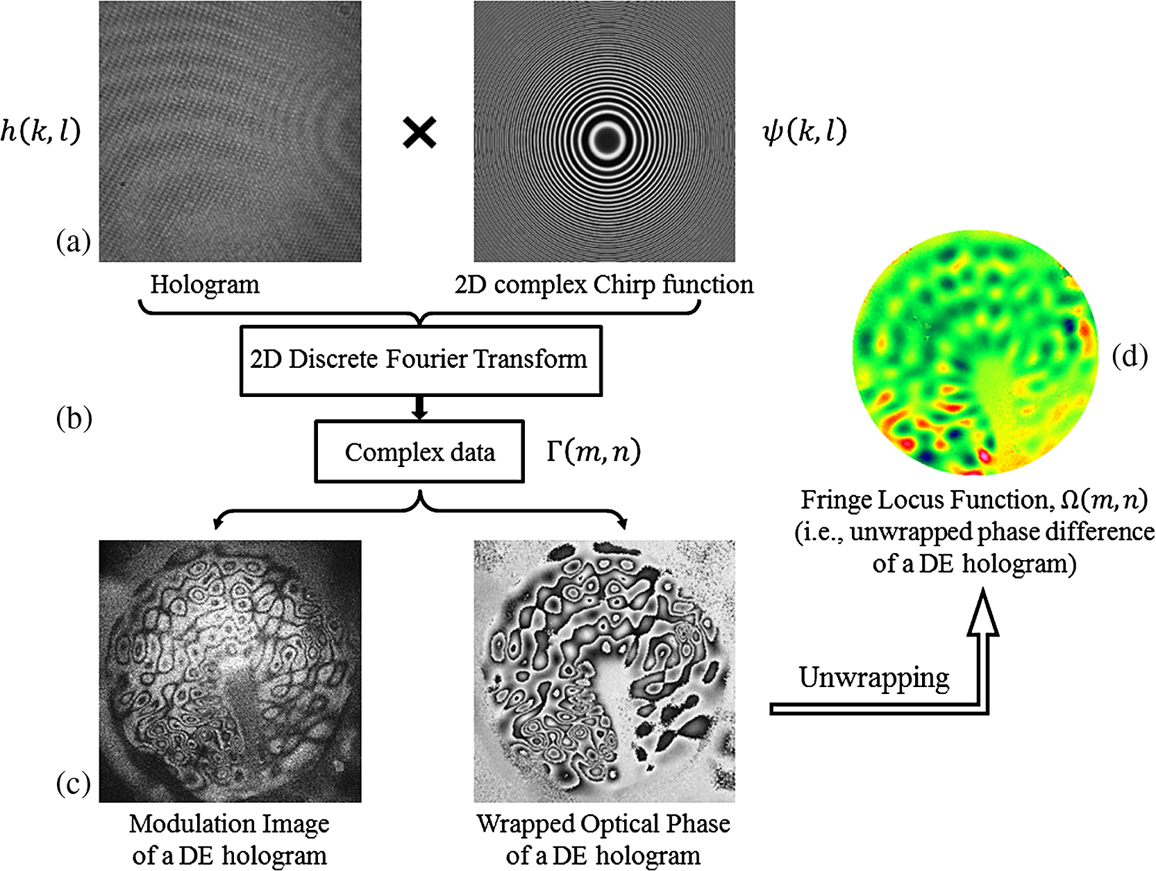$\mathrm{\Omega }(m,n)$.

The fringe-locus function of a double-exposure (DE) hologram, i.e., the unwrapped optical phase difference of two reconstructed holograms corresponding to deformed and reference states of the object, is related to displacement with^15,16

2.2.

Stroboscopic Measurements of Displacement

Sound-induced vibrations of the TM are fast phenomena that require high-speed acquisition methods to be captured. In our system, we use stroboscopic measurements^17–21 with a conventional speed camera to capture the repetitive fast motions produced by sinusoidal stimuli. Acoustically induced motions of the TM are frozen at different stimulus phases using pulses of laser light to illuminate the sample at particular points during the sinusoidal excitation signal. As shown in Fig. 2, a dual-channel function generator is used with one of the channels set to a sine wave for stimulating the TM through a speaker. The second channel is set to the same frequency but with a pulse wave to drive an acousto-optic modulator (AOM) to enable and disable the laser beam illumination. Typically, each laser pulse has a duration of 2% to 5% of the period of the tonal stimulus.^11,18 This generates the same effect as a strobe light by only capturing the motion of the TM at desired phases of the stimulus wave.

Fig. 2

Signals for stroboscopic measurements of sound-induced displacements of the TM at an example phase of 90 deg: (a) sinusoidal signal sent to the speaker to stimulate the TM and (b) pulsed signal sent to the acousto-optic modulator (AOM) that acts as a high-speed shutter for laser light illumination with a duty cycle of 2% to 5% of the tonal excitation period. During a full measurement, the phase position of the pulse is varied from 0 to 360 deg at specified increments to enable capturing of the entire cyclic motion.

A DE technique that compares the deformed state strobe hologram gathered at one phase and a hologram gathered at a reference phase (usually 0) is used to compute the displacement of a series of strobe holograms to describe the phase-locked sound-induced variation in the optical phase. The result is a wrapped phase map that describes the differences in optical phase between the deformed and reference states. At every DE strobe hologram, including reference and deformed states, the system records four images containing holographic patterns that result from the phase stepping of the reference beam (RB) in steps of multiples of $\pi /2$. Considering the intensities at each pixel measured by the camera at each of the four phase steps to be $I_1,\dots ,I_4$ in the reference state, and $I_1^{\prime },\dots ,I_4^{\prime }$ in the deformed state, the wrapped optical phase difference between any two states is related to displacements of the sample and is obtained with

2.3.

Dual-Wavelengths Shape Measurement

The shape of the TM is measured with the method of dual-wavelength holographic contouring.^22,23 The technique requires acquisitions of a set of optical amplitude and phase information at wavelength ${\lambda }_1$, as well as a second set of amplitude and phase information at wavelength ${\lambda }_2$. As shown in Fig. 3, depth contours related to the shape of the object under investigation are defined by

Fig. 3

Optical path length (OPL) of the laser light in dual-wavelength holographic contouring. $P_1$ is the point of illumination, $P_2$ is the point of observation, and $P$ is a point on the surface of the object of interest. Surfaces of constant optical phase intersect the object of interest generating contours of depth $h$.

The phase difference obtained with Eq. (8) is equivalent to performing measurements with a synthetic wavelength of $\mathrm{\Lambda }$ given by

In dual-wavelength contouring using phase-stepping algorithms, the phase difference, $\mathrm{\Delta }\varphi$, is a discontinuous wrapped function varying in the interval $[-\pi ,\pi ]$, thus phase unwrapping algorithms are applied to obtain a continuous phase distribution, $\mathrm{\Omega }(m,n)$, for calculation of the relative height of each point on the surface of the object $Z(m,n)$ by

2.4.

3-D Displacement Measurements

To ensure that measurements are reliable and independent of the measuring method, the holographic system is configured so that principal components of displacements, ${\mathit{d}}_x$, ${\mathit{d}}_y$, ${\mathit{d}}_z$, can be measured with two different holographic interferometric approaches. The first one is based on the method of multiple illumination directions, whereas the second one uses a hybrid in-plane and out-of-plane displacement measurement method to obtain 3-D displacement data. In the hybrid method, in-plane measurements provide displacements’ components along the $x$- and $y$-axes (perpendicular to the observation direction) and out-of-plane measurements provide displacements’ components along the $z$-axis (along the observation direction).

2.4.1.

Method of multiple illumination directions

Full field-of-view, 3-D, sound-induced displacements of the TM are measured with the method of multiple illumination directions in holographic interferometry.^24,25 In order to measure the three components of the displacement vector, $\mathit{d}$, shown in Eq. (6), at least three independent measurements with different sensitivity vectors are required. In our approach, and to minimize experimental errors,^24,26 optical phase maps are obtained with four sensitivity vectors to form an over determined system of equations that is solved in Matlab with the least-squares error minimization method with

Eq. (12)

$$\{\mathit{d}\}={[{[\mathbb{S}]}^T[\mathbb{S}]]}^{-1}\times \{{[\mathbb{S}]}^T\{\mathrm{\Omega }\}\},$$

where $[\mathbb{S}]$ is the sensitivity matrix containing all the sensitivity vectors ${\mathit{K}}_i$, shown in Fig. 4, and $\{\mathrm{\Omega }\}$ is the fringe-locus function vector. In this method, all the sensitivity vectors need to be as linearly independent as possible for the system to provide accurate results. Therefore, the condition number, $\mathbb{C}$, of the square matrix, $[F]={[\mathbb{S}]}^T[\mathbb{S}]$, characterizing the geometry of a holographic setup is calculated with²⁷

Eq. (13)

$$\mathbb{C}(\mathbb{S})=\sqrt{\frac{{\lambda }_{\max }(F)}{{\lambda }_{\min }(F)}},$$

where ${\lambda }_{\max }$, and ${\lambda }_{\min }$ are the maximum and the minimum eigenvalues of $[F]$. A condition number close to one indicates a well-conditioned matrix, but this represents a holographic setup with large angles of illumination.^15,28 However, because of the particular cone-like geometry of the TM and the presence of the bony structures around it, as illustrated in Fig. 4, the maximum possible angles of illumination are limited. Therefore, a holographic setup has to be arranged to achieve the largest angles of illumination within the constraints imposed by the geometry of the TM. In this case, the condition number is greater than one, therefore, the accuracy of the measurements obtained with such a holographic setup has to be verified.

Fig. 4

3-D displacement measurements of the TM surface by the method of multiple illumination directions. Sensitivity vectors for each illumination direction, ${\mathit{K}}_i$, are obtained by vectorial subtraction of the corresponding unit observation vector, ${\mathit{K}}_2$, from the unit illumination vector, ${\mathit{K}}_{1i}$. The geometry of the TM limits the maximum angle of illumination that can be implemented to achieve a well-conditioned sensitivity matrix.

2.4.2.

Hybrid in-plane and out-of-plane method

A hybrid method that utilizes independent and direct measurements of “out-of-plane” and “in-plane” displacements is used to test and verify the measurements obtained with the method of multiple sensitivity vectors. In this hybrid method, in-plane measurements provide displacement components along the $x$- and $y$-axes (perpendicular to the observation direction), and out-of-plane measurements provide displacements along the $z$-axis (along the observation direction), so that all three displacement components can be obtained independently.

Figure 5 shows optical configurations of the two measuring schemes. As shown in Fig. 5(a), an out-of-plane displacement $d_{\text{out}}$ induces a change in the OPL of the laser light (OPD). Based on the geometry of the system, OPD is related to the out-of-plane displacement $d_{\text{out}}$ with

Eq. (14)

$$\mathrm{OPD}=d_{\text{out}}\cos ({\theta }_1),$$

where ${\theta }_1$ is the angle between the illumination and observation directions. Using the wavenumber equation, $k=2\pi /\lambda$, OPD is converted to the out-of-plane fringe-locus function, ${\mathrm{\Omega }}_{\text{out}}$, with ${\mathrm{\Omega }}_{\text{out}}=(2\pi /\lambda )\mathrm{OPD}$, and consequently, the out-of-plane displacement $d_{\text{out}}$ is calculated with

Eq. (15)

$$d_{\text{out}}=\frac{\lambda {\mathrm{\Omega }}_{\text{out}}}{2\pi [1+\cos ({\theta }_1)]}.$$

Fig. 5

Two displacement measurement schemes that are combined to achieve 3-D displacement measurements in the hybrid method: (a) configuration for out-of-plane (along $z$-axis) displacement measurements and (b) configuration for in-plane (along $x$- or $y$-axes) displacement measurements. The dashed lines represent illuminations after displacement occurs. OPD is OPL difference.

In the case of in-plane measurements, the object is illuminated with two symmetrical beams that interfere with each other and realize a self-reference configuration.²⁹ As shown in Fig. 5(b), once in-plane displacement, $d_{\text{in}}$, occurs, the OPL of each interfering beam changes, which causes a relative phase change between the two interfering beams. Figure 5(b) shows only one of the in-plane components of displacement, however, displacement components along both the $x$- and $y$-axes are independently measured with this method.

Equations (16) and (17) show the relation between OPD and the in-plane fringe-locus function corresponding to the in-plane displacement $d_{\text{in}}$

Eq. (16)

$${\mathrm{OPD}}_1={\mathrm{OPD}}_2=d_{\text{in}}\cos (\frac{\pi }{2}-\theta )=d_{\text{in}}\sin (\theta ),$$

Eq. (17)

$${\mathrm{\Omega }}_{\text{in}}=\frac{2\pi }{\lambda }({\mathrm{OPD}}_{\text{total}}),$$

where ${\mathrm{OPD}}_{\text{total}}={\mathrm{OPD}}_1+{\mathrm{OPD}}_2$. Using Eqs. (16) and (17), in-plane displacement, $d_{\text{in}}$, is calculated with

Eq. (18)

$$d_{\text{in}}=\frac{\lambda {\mathrm{\Omega }}_{\text{in}}}{4\pi \sin (\theta )},$$

where ${\mathrm{\Omega }}_{\text{in}}$ is the in-plane fringe-locus Function, $\lambda$ is the wavelength of the laser, and $\theta$ is the angle between the illumination and observation directions.

2.5.

Experimental Setup

The schematic of the developed Digital Opto-Electronic Holographic System (DOEHS) is shown in Fig. 6. The DOEHS can measure microscale variations in shape as well as nanoscale displacements of the TM using both 3-D displacement measurement methods described in Sec. 2.4. The DOEHS consists of three main subsystems including laser delivery (LD), computing platform (CP), and optical head (OH). An external-cavity tunable diode laser capable of continuous tuning with minimal mode hopping (New Focus, Velocity) is placed in the LD, which provides a near IR laser light with a central wavelength of 780 nm. A polarization maintaining fiber coupler (Thorlabs PM-780-HP) splits the light into two beams to be used as reference (10%) and object (90%) beams. A MEMS optical switch, with a response time of less than 0.5 ms (Thorlabs OSW 8104), is used to multiplex between the object beams (OB) of each illumination direction once triggered by a Digital to Analog signal. The CCD is illuminated with the RB through a beam splitter and through a piezo-mounted mirror that is used for phase stepping. A 5 Megapixel ($2452\times 2054\text{pixels}$) digital camera with a pixel pitch of $3.45\mu \mathrm{m}$ in the OH is used for image recording and the CP acquires and processes images in either time-averaged or DE stroboscopic modes.³⁰ The sinusoidal output of the function generator is amplified by a unity gain power amplifier and is used to drive the speaker. A microphone with a calibrated probe tube was positioned just at the edge of the TM to make measurements of sound pressure. In stroboscopic measurements, the light illumination is synchronized with the sound-waveform by means of a digital pulse signal from the function generator to the AOM.

Fig. 6

Schematic of the developed holographic system for shape and 3-D displacement measurements. The laser delivery (LD) subsystem consists of a near-infrared tunable laser (with central wavelength of 780 nm), acousto-optic modulator (AOM), mirror, and laser to fiber coupler; the computing platform (CP) controls the recording parameter such as sound-excitation frequency and sound pressure level, phase-stepping, synchronizations for stroboscopic measurements, and controlling the optical switch (OS) for high-speed multiplexing between any of the object beams (OB1-OB4). The dashed lines are analog and digital signal lines.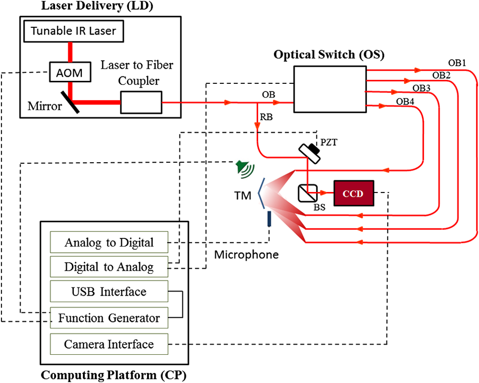

2.6.

Determination of the Sensitivity Vectors

In the method of multiple illumination directions, accurate determination of the position of each illumination source is required to define the corresponding sensitivity vectors. A new technique is developed in which all the sensitivity vectors are obtained by automatic analyses of the images of a specular sphere illuminated from different directions in order to avoid the uncertainties introduced by manual measurements. As shown in Fig. (7), a specular sphere is placed in front of the imaging system to acquire images from all four directions of illumination. The center of the image is marked in the acquisition software LaserView³⁰ and the sphere is accurately located in this position and within a circular mask provided by the software to ensure that the sphere is placed along the optical axis of the holographic system. As shown in Fig. 7(a), the mirror-like reflection creates a specular highlighted area on the sphere.³¹ Each image is cropped and enhanced by image processing techniques that include histogram equalization, threshold definition, and edge detection. Then, a sphere is numerically fitted on the detected circular edge which represents the outline of the sphere. The normal vector of the fitted sphere at the centroid of the specular highlighted area, for each direction of illumination, defines the sensitivity vector, ${\mathit{K}}_i$, which can be expressed as

Fig. 7

Automatic determination of a sensitivity vector by use of a specular reflective sphere and circular Hough transformation (CHT): (a) image of a specular reflective sphere illuminated with one of the object beams, (b) cropped, enhanced image of the sphere, (c) CHT algorithm is used to detect the specular highlighted area and its centroid, and (d) the normal vector at the centroid of the detected highlighted area defines the sensitivity vector.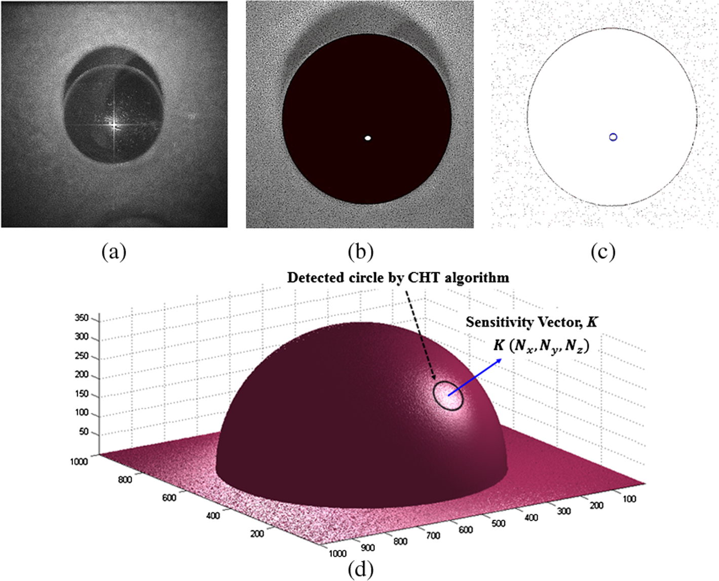

3.1.

Validation of Measuring Accuracy and Repeatability

Considering the acquisition speed of the 3-D holographic system and the time-dependent mechanical behavior of biological samples like the TM, we characterized the accuracy and repeatability of the measurements of the 3-D holographic system using measurements of artificial samples that have negligible time-varying behaviors. Based on the particular concave shape of the TM, a semispherical membrane with a geometry similar to the TMs is used. For 3-D displacement measurements of non-flat membranes, the large illumination angles necessary for a well-conditioned 3-D holographic system create shadows on the surface of the membrane. Therefore, the maximum angles of illumination are limited by geometrical constraints induced by the membrane, leaving the holographic system with condition numbers greater than one, as described in Sec. 2.4.1. To calibrate the measuring system and to verify the accuracy of the measurements obtained with such non-ideal 3-D holographic configuration, 3-D displacement components are measured using both of the methods described in Sec. 2.4, in order to ensure that the obtained displacement components are accurate and independent of the measuring approach. Once the accuracy of the measurements is verified, repeatability of the stroboscopic measurements is tested and verified with sound-induced displacement measurements of a latex membrane.

3.1.1.

Accuracy of 3-D displacement measurements

The shape and 3-D displacements of a thin semispherical membrane, shown in Fig. 8, with a radius of 6 mm and a thickness of $25\mu \mathrm{m}$ are measured with the developed holographic system. The shape of the membrane is measured with a dual-wavelength contouring method with wavelengths of 779.8 and 780.6 nm. Figure 8(b) shows the wrapped optical phase, which is unwrapped and scaled to obtain the corresponding 3-D shape, as shown in Fig. 8(c).

Fig. 8

Measurements of the shape of an artificial membrane using dual-wavelength holographic contouring: (a) semi-spherical membrane with a thickness of $25\mu \mathrm{m}$ and a radius of 6 mm, (b) wrapped optical phase corresponding to the shape of the membrane, and (c) 3-D scaled shape of the membrane.

The semispherical membrane is mounted on a piezoelectric shaker (JODON EV-100) that can operate at frequencies as high as 150 kHz. By sweeping the excitation frequency and monitoring the membrane’s time-averaged motions,^10,16,33 an appropriate mode of vibration is chosen. Representative results are shown in Fig. 9, in which the membrane is excited with a frequency of 25,418 Hz and amplitude of 0.4 V. Comparisons of the displacement components along the $x$-, $y$-, $z$-axes, and the magnitudes of displacements obtained with both methods show correlation coefficients $>95\%$, illustrating that the measurements are accurate, repeatable, and independent of the measuring method.

Fig. 9

3-D displacement components of a semi-spherical membrane excited mechanically with a piezoelectric shaker at a frequency of 25,418 Hz. Displacement components measured with the method of multiple illumination directions along (a) $x$-axis, (b) $y$-axis, (c) $z$-axis, (d) magnitude of displacement, and displacement components measured with the hybrid method along (e) $x$-axis, (f) $y$-axis, (g) $z$-axis, (h) magnitude of displacement. The correlation coefficient, $\mathbb{R}$, of the displacements component obtained with the two methods are 0.95, 0.96, 0.99, and 0.99 for displacement components along $x$-, $y$-, $z$-axes, and magnitude of displacement, respectively. All the displacements are in micrometers.

3.1.2.

Repeatability of stroboscopic measurements

Repeatability of the results obtained with the 3-D holographic system is tested and verified by a series of consecutive stroboscopic measurements of a 10 mm diameter latex membrane excited with a tone of 2917 Hz at 91 dB sound pressure level (SPL), as shown in Fig. 10. Figures 10(a)–10(c) show representative examples of the obtained modulation, wrapped optical phase, and magnitude of displacements, respectively. Furthermore, repeatability of the measurements is shown in Fig. 10(d), where vertical (shown with dashed lines) and horizontal (shown with solid lines) cross-sections of six consecutive displacement measurements lie on top of each other.

Fig. 10

Repeatability of the holographically obtained displacement measurements of a circular latex membrane acoustically excited with a tone of 2917 Hz at 91 dB SPL along one sensitivity vector. Representative DE (a) modulation, (b) wrapped optical phase, (c) map of the magnitudes of displacements averaged over six consecutive measurements, and (d) cross-sections of six displacement maps along specific horizontal (solid) and vertical lines (dashed), illustrating the repeatability of the measurements.

3.2.

Shape and 3-D Sound-Induced Displacements of Human TM

The TM sample was part of a human right ear temporal bone from a 49-year-old male donor. The sample was prepared in accordance with previously established procedures.^9,12 In order to have the least amount of shadow on the surface of the TM, all the bony structures around the TM were removed. In preparing the specimen, it was necessary to also open the middle ear cavity, however, those openings were filled by silicone impression materials (Westone Inc.) prior to these measurements in order to avoid and minimize the air flow through the middle ear cavity. Also, to enhance light reflection from the sample and to reduce the required camera exposure time in order to have a better signal to noise ratio, the lateral surface of the TM was coated with a solution of zinc oxide. The effect of this coating on the vibrational patterns of the TM has been shown to be negligible.^9–11 The shape of the sample was measured with dual-wavelength holographic contouring, as shown in Fig. 11, with two wavelengths of 780.2 and 780.6 nm. Figure 11(b) shows the wrapped optical phase, which is unwrapped and scaled to obtain corresponding 3-D shape, as shown in Fig. 11(c).

Fig. 11

Measuring the shape of a human tympanic membrane (TM) using dual-wavelength holographic contouring: (a) human temporal bone highlighting the tympanic ring, (b) wrapped optical phase corresponding to the shape of the TM, and (c) 3-D shape of the TM. The shape is measured with wavelengths of 780.2 and 780.6 nm.

Tones with different frequencies were used to stimulate the membrane and 3-D sound-induced displacement components of the surface of the TM were acquired. Figure 12 shows 3-D displacement components of the TM along the $x$-, $y$-, and $z$-axes produced by tones of 1560 Hz at 108 dB SPL, 4480 Hz at 101 dB SPL, and 8021 Hz at 96 dB SPL. The levels were selected to generate measurable sound-induced TM displacements. As shown in Fig. 12, as sound excitation frequency increases, the number of local maxima in the displacement patterns also increases and sound-induced motion patterns of the TM become more complex.

Fig. 12

Measured 3-D sound-induced displacement of a human TM along the $x$-, $y$-, and $z$-axes at three different tonal excitations. Magnitudes of displacements along $x$-, $y$-, and $z$-axes are (a) $\pm 220$, $\pm 250$, and $\pm 520\mathrm{nm}$ for tonal frequency of 1560 Hz at 108 dB SPL, (b) $\pm 200$, $\pm 120$, and $\pm 220\mathrm{nm}$ for tonal frequency of 4480 Hz at 101 dB SPL, and (c) $\pm 110$, $\pm 210$, and $\pm 510\mathrm{nm}$ for tonal frequency of 8021 Hz at 96 dB SPL. The diameter of the TM is 8 mm and the outline shows the handle of malleus (manubrium).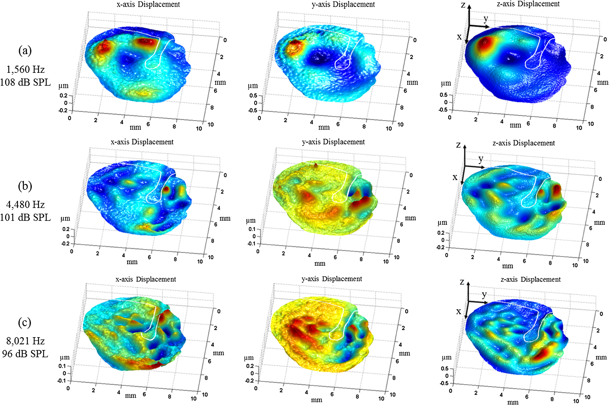

Combining data obtained from the shape of the membrane, shown in Fig. 11, with measured 3-D sound-induced displacement components, shown in Fig. 12, displacement components tangent (in-plane) and normal (out-of-plane) to the TM surface are obtained. A numerical rotation matrix is used³⁴ to rotate the original Euclidean coordinate system of the measuring system $(x,y,z)$, so that the new coordinate system $(\alpha ,\beta ,\eta )$ has unit vectors tangent and normal to the TM surface. Figure 13 shows the results of the rotation of the coordinate system, where rotated displacements have components tangent (in-plane components $d_{\alpha }$ and $d_{\beta }$), and normal to the TM surface (out-of-plane component $d_{\eta }$). As shown in this figure, in-plane components are much smaller than out-of-plane components ($<20\%$), so that the displacement vectors can be considered to be mainly normal to the surface of the TM.

Fig. 13

In-plane and out-of-plane sound-induced motions of a human TM excited with frequency of (a) 1560 Hz at 108 dB SPL, (b) 4480 Hz at 101 dB SPL, and (c) 8021 Hz at 96 dB SPL. It can be clearly seen that tangential (in-plane) components are negligible and the motions are mainly normal (out-of-plane) to the TM surface. Displacements are in the unit of micrometers.

These data support hypotheses based on considering the motions of the TM similar to those of thin-shells, in which the tangential motions’ components are negligible and the motion vectors are hypothesized to be mainly along the normal vector of the surface of the membrane.^8,9