|
|
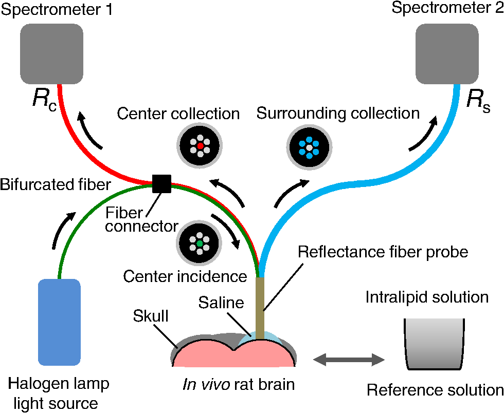
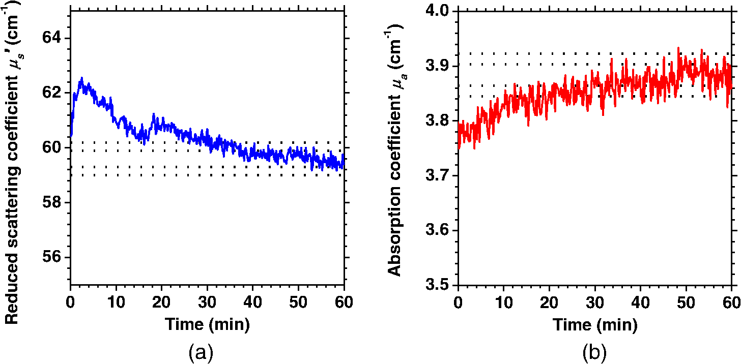
1.IntroductionCortical spreading depression (CSD) is a wave of neuronal and glial depolarization propagating in 2 to 4 mm/min over the cerebral cortex.1–3 CSD is an important disease model for migraine4 and is related to other neurological disorders, such as neurotrauma,5 seizure,6 and ischemia.7,8 CSD initiated in vivo has been discussed in terms of the changes in tissue optical properties related to hemodynamics originating from neurovascular coupling in brain tissue. Cerebral blood flow during CSD in small animals has been investigated by laser speckle flowmetry,9 laser Doppler flowmetry,10 and the diffuse optical correlation method.11 On the other hand, diffuse reflectance imaging with single or multiple wavelengths has suggested that during CSD, changes in light scattering occur due to cell deformation in tissue.12–14 In order to investigate the relationship between CSD and clinical disorders, it is important to evaluate the changes in the optical properties of in vivo brain due to both hemodynamics and the tissue itself. The optical properties of biological tissue have been used to evaluate spatial and/or temporal changes of physiological and morphological conditions in living tissues. Changes in the optical properties of the tissue occur primarily due to the following processes: hemodynamic-related changes in absorption and scattering, changes in absorption due to redox states of cytochromes in mitochondria, changes in scattering generated by cell swelling or shrinkage due to the movement of water between intracellular and extracellular compartments,15 and changes in scattering and absorption caused by chromophore content and cell deformation. Light in the visible to near-infrared (NIR) spectral range is sensitive to the absorption and scattering properties of biological tissue. The absorption and scattering properties of in vitro tissue slices can be estimated from the measured diffuse reflectance and transmittance of tissue slices16 based on several light transport models, such as the Kubelka-Munk theory,17 diffusion approximation to the transport equation,18 the Monte Carlo method,19 and the adding-doubling method.20 A number of spectroscopic methods have been studied for in vivo determination of the scattering and absorption properties in living tissues, including time-resolved measurements,21 a frequency-domain method,22 and spatially resolved measurements.23–27 Diffuse reflectance spectroscopy (DRS) based on spatially resolved measurements with a continuous-wave light can be simply achieved using a white light source, inexpensive optical components, and a spectrometer. An optical fiber is generally used to deliver the illumination light to and collect the diffusely reflected light from in vivo tissue for DRS instruments, as well as endoscopes and colposcopes.28 DRS using a fiber optic probe is a promising technique for monitoring tissue oxygenation, distinguishing between normal and malignant tissues,29 and assessing tissue viability.30 Various source-collector geometries have been used to estimate the reduced scattering coefficient, , and the absorption coefficients, , in DRS using a fiber optic probe.23,29,31–34 In general, the sampling volume increases as the source-collector separation increases. However, large sampling volumes are likely to be inhomogeneous. Therefore, when measuring the optical properties of a local volume, it is desirable to use a small source-collector separation. Moreover, a single-reflection probe will be easy to use in practical applications, especially in clinical situations. In the present study, we propose a method by which to determine the reduced scattering coefficients, , and the absorption coefficients, , of in vivo biological tissue based on DRS using a single-reflectance fiber probe with two source-collector geometries. In order to confirm the validity of the proposed method in evaluating changes in the optical properties of the cerebral cortex evoked by CSD, we performed in vivo experiments using exposed rat brain during CSD evoked by topical application of KCl. 2.Principle2.1.Reflectance Fiber Probe SystemFigure 1 shows a schematic diagram of the single-reflectance fiber-probe system with the two source-collection geometries used in the present study. The system consists of a light source, bifurcated fiber, a reflectance fiber probe, and two spectrometers under the control of a personal computer. The bifurcated fiber has two fibers of the same diameter of side-by-side in the common end. The reflectance fiber probe has one fiber in the center surrounded by six fibers. The common end of the bifurcated fiber is connected to one end of the center fiber of the reflectance probe by a fiber connector. A halogen lamp light (HL-2000, Ocean Optics Inc., Dunedin, Florida, USA), which covers the visible-to-NIR wavelength range, is used to illuminate the sample via one lead of bifurcated fiber and the central fiber of the reflectance probe. Diffusely reflected light from the sample is collected by the central fiber and the six surrounding fibers. The center-to-center distances between the central fiber and the surrounding fibers are . The light collected by the central fiber is delivered to a multichannel spectrometer (USB4000, Ocean Optics Inc.) via another lead of the bifurcated fiber, whereas that collected by the six surrounding fibers is delivered to a different multichannel spectrometer (USB4000, Ocean Optics Inc.). A solution of Intralipid 10%35 was prepared as a reference solution. Diffuse reflectance spectra and were calculated from the spectral intensities of light collected by the central fiber and the six surrounding fibers, respectively, based on the reflected intensity spectra from the reference solution. 2.2.Monte Carlo Simulation of Light Transport in TissueIn order to estimate the absorption coefficient and the reduced scattering coefficient based on the measured diffuse reflectance, we performed Monte Carlo simulations for light transport using the source-collection geometries of the reflectance fiber probe shown in Fig. 1. Figures 2(a) and 2(b) show the simulation models for and , respectively. Each simulation model consists of a fiber and a sample. We used the Monte Carlo simulation code developed by Wang et al.,19 in which the Henyey-Greenstein phase function is applied to a sampling of the scattering angle of photons. The source code was modified for the two source-collection fiber configurations. The source and collection areas were located on the boundary between the fiber and the scattering medium. The source and collection areas were identical in the simulation model for [Fig. 2(a)]. The distance between the source and collection fiber areas was in the simulation model for [Fig. 2(b)]. In a single simulation, 1,000,000 photons were randomly launched uniformly within the radius of the source fiber. Photons were launched with equal probability over the entire face of the source fiber and were propagated into the medium under scattering and absorption. Then, a portion of the scattered light returns from the medium and is finally emitted from the surface of the medium. For all of the simulations, the refractive index of the fiber, , and that of the medium, , were fixed at 1.458 and 1.4, respectively. Only photons that had an angle less than or equal to the maximum acceptance angle and passed back through the face of collection fiber were counted into the collected light intensity. In order to estimate collected by all of the surrounding fibers, the diffuse reflectance simulated by the multiple-fiber geometry shown in Fig. 2(b) is multiplied by 6. In the Monte Carlo simulations, and were calculated for the ranges of to and to . Figures 3(a) and 3(b) show the results obtained from the Monte Carlo simulation for and , respectively. The value of increases monotonically as increases, whereas reaches a plateau for larger values of . Both and decrease exponentially as increases, but the effect is more pronounced for . Fig. 2Schematic diagram of the Monte Carlo simulation models that represents the fiber configurations of the reflectance probe used in the present study. (a) Single-fiber configuration in which a central fiber of the reflection probe is used both as the source and for collection of light. (b) Multiple-fiber configuration in which the central fiber is used as the source and the surrounding fibers are used for collection of light.  2.3.Determination of Empirical Formulas for Estimating andIn order to estimate and from the measurements of and , we consider the following empirical equation based on the results of the Monte Carlo simulation: where and are the apparent absorbances for the recording by the center fiber and surrounding fibers, respectively. In order to improve the accuracy of Eq. (1), we used the higher-order terms of and in Eq. (1) as follows: where coefficients and (, 1, 2, 3, 4, 5) in Eq. (2) can be determined statistically by multiple regression analysis of the results of the Monte Carlo simulations, and represents the transposition of a vector. The values of and can be estimated by applying Eq. (2) to each wavelength point of and . Figure 4 shows the estimated and expected values of the reduced scattering coefficient [Fig. 4(a)] and the absorption coefficient obtained from the preliminary numerical investigations [Fig. 4(b)]. In both Figs. 4(a) and 4(b), the estimated values well agree with the expected values for given ranges of and . The values for and were 0.99 and 0.99, respectively, which indicates a good regression.2.4.Calculation of Tissue Oxygen Saturation fromThe absorption coefficient spectrum is given by the sum of absorption due to oxygenated and deoxygenated hemoglobin as follows: where is the concentration and is the extinction coefficient spectrum. Subscripts HbO and Hb denote oxygenated hemoglobin and deoxygenated hemoglobin, respectively. The oxygen saturation of hemoglobin, , is defined by the concentrations of oxygenated and deoxygenated hemoglobin as follows:Using the absorption coefficient spectrum as a response variable and the extinction coefficient spectra of and 26 as predictor variables, the multiple regression model can be applied to Eq. (3) as follows: where , , and are the regression coefficients, is an error component, and indicates discrete values in the wavelength range treated in the analysis. By executing the multiple regression analysis for one sample of the absorption coefficient spectrum consisting of discrete wavelengths, one set of the three regression coefficients is obtained. In the present study, we used the spectral data in the range from 500 to 600 nm at intervals of 10 nm for the multiple regression analysis because the spectral features of oxygenated and deoxygenated hemoglobin notably appear in this wavelength range. The regression coefficients and describe the degree of contributions of and , respectively, to the absorption coefficient spectrum and, consequently, are closely related to the concentrations and , respectively. The oxygen saturation was estimated from the regression coefficients and as follows:3.Experiments3.1.Validation of the Proposed Method Using Optical PhantomsBefore the in vivo experiments, preliminary experiments were carried out using optical phantoms. The phantoms were prepared using Intralipid stock solution (Fresenius Kabi AB, Sweden) as scattering materials and hemoglobin solution extracted from red blood cells of horse blood as the absorber. We prepared the scattering solutions by diluting Intralipid stock solution with saline. The absorption coefficients of hemoglobin were experimentally determined based on the transmittance measurements of hemoglobin solutions within a cuvette using a spectrometer. The reduced scattering coefficients of Intralipid solutions were evaluated based on the published values.35 We first produced 12 phantoms with ranges of to and to in the wavelength range from 500 to 900 nm to compare the estimated and given optical properties. We also performed the phantom experiments based on the standard protocols developed within the European Thematic Network MEDPHOT (optical methods for medical diagnosis and monitoring of diseases).36 The MEDPHOT protocol is composed of five criteria: accuracy, linearity, noise, stability, and reproducibility. The accuracy of the measurement is defined as the capacity of the instrument for obtaining a value for the measurable value as close as possible to the conventionally true value . In the accuracy assay, the crosstalk in the estimation of and can also be investigated by the results of experiments in which is estimated when only changes and vice versa in order to evaluate how much a change in an optical property interferes with the estimation of the other property. A linearity assay was performed by measurement of a set of phantoms combining five values for the hemoglobin concentration, with three values for the concentration of Intralipid solution to check whether the system can follow changes in given values of and without distortions. The noise assay was performed by repeating a series of measurements on the same phantom. We investigated the coefficient of variation CV of a certain number of repeated measurements against the injected energy as follows: where is the standard deviation for a measurable value , calculated for a series of repeated measurements, and is the corresponding average value. The plot of can be used to evaluate the minimum energy that must be injected in the sample to obtain a fluctuation of the measurement below a certain threshold. The stability assay was performed by repetition of the measurement on the same phantom many times at subsequent time instants without changing the experimental conditions. The reproducibility assay was performed by repetition of the measurement on the same phantom under the same experimental conditions on different days.A total of 15 phantoms were constructed by combining three concentrations of Intralipid solution with five concentrations of hemoglobin. These phantoms were labeled with a letter and a number, in which the letter stands for the scattering (, , and corresponding to , 40.2, and , respectively) and the number indicates the absorption (1, 2, 3, 4, and 5 corresponding to , 1.25, 1.5, 1.75, and , respectively). In addition, one more phantom was constructed for the reproducibility assay by the combination of a polystyrene latex beads solution and hemoglobin and with identical values of and at 500 nm. The reflectance fiber probe was inserted vertically within the phantoms to a depth of from the surface. The face of the reflectance fiber probe was pointing toward the bottom of the container. 3.2.Animal ExperimentsThe animal care and experimental procedures of this study were approved by the Animal Research Committee of Tokyo University of Agriculture and Technology. Intraperitoneal anesthesia was implemented using a mixture of -chloralose () and urethane () in nine male Wister rats (80 to 286 g). Anesthesia was maintained at a depth such that the rat had no response to toe pinch. The rat head was placed in a stereotaxic frame. Figure 5(a) shows a schematic diagram of the measurement area and the stimulation sites on the rat head. A longitudinal incision long was made along the head midline. The skull bone overlying the parietal cortex was removed using a high-speed drill to form an ellipsoidal cranial window (major axis: 8.0 mm, minor axis: 6.0 mm). The cranial window was bathed with normal saline. The end of the reflectance fiber probe was placed on the exposed cortex with care taken to avoid large blood vessels. A burr hole (diameter: 2 mm) was drilled in the ipsilateral frontal bone as a site for contacting the cortex with a 3 M KCl solution. The center-to-center distance between the burr hole and the reflectance fiber probe was 9.3 mm. CSD was induced by applying a droplet of the KCl solution to the burr hole. The extracellular local field potential (LFP) was recorded using a single Ag/AgCl electrode with a ball-shaped tip (tip diameter: 1 mm). The recording electrode was placed on the cortex anterior to the edge of the reflectance fiber probe with care taken to avoid large blood vessels. The center-to-center distance between the burr hole and the recording electrode was 6.9 mm on average. An Ag/AgCl reference electrode (RC5, World Precision Instruments Inc., Sarasota, Florida, USA) was placed in the neck muscle. Figure 5(b) shows a schematic diagram of the experimental setup. Measurements of and were obtained simultaneously in the wavelength range of 500 to 900 nm at 10 s intervals for 50 min. The KCl solution was applied to the cortical surface through the burr hole 1 min after the onset of measurement and was washed out 16 min after the onset of measurement. The LFP signal was amplified at 1 to 100 Hz using a differential amplifier (DAM50, World Precision Instruments Inc.) and was digitized at 5 Hz using an oscilloscope (TDS1000C-EDU, Tektronix) connected to a personal computer running Open Choice software. Fig. 5Schematic diagram of (a) measurement and stimulation sites on the rat head and (b) experimental setup for in vivo rat brain during cortical spreading depression. 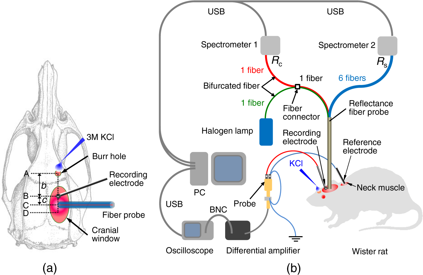 Since the proposed method requires the fiber probe to be in contact with the surface of the exposed brain, it is difficult to measure the LFP signal at the same position as the reflectance fiber probe. Therefore, we estimate the time of the negative peak of the LFP at a position under the reflectance fiber probe as the arrival time of CSD. First, the propagation speed of CSD, (mm/min), is calculated as follows: where (mm) is the distance between the position at which the KCl solution is in contact with the brain surface and the Ag/AgCl recording electrode, and (min) is the time interval between the application of KCl, , and the first negative peak of LFP, . The propagation time of CSD between the Ag/AgCl recording electrode and the reflectance fiber probe, (min), is then calculated as follows: where (mm) is the distance between the Ag/AgCl recording electrode and the reflectance fiber probe. Finally, the estimated time of the negative peak of LFP at a position under the reflectance fiber probe, (mm), can be estimated as follows: where (min) is the onset of KCl application. The estimated arrival time of CSD at the position under the reflectance fiber probe is compared with the time courses of , , and . In order to investigate the effects of changes in electrode position on the estimated time of the negative peak of LFP, we also performed the measurements of LFPs with two recording electrodes for one rat. In this case, recording electrode 1 was placed on the cortex anterior to the edge of reflectance fiber probe [position B in Fig. 5(a)], whereas recording electrode 2 was placed on the cortex posterior to the edge of reflectance fiber probe [position D in Fig. 5(a)].4.Results and Discussion4.1.Validation of the Proposed Method Using Optical PhantomsFigure 6 shows the estimated and given values for the reduced scattering coefficient [Fig. 6(a)] and the absorption coefficient [Fig. 6(b)]. Reasonable results were obtained for both and . Correlation coefficients between the estimated and given values are () and () for and , respectively. The average root mean square error for is and that for is . The proposed method yields, in principle, good results for both and , as shown in Figs. 4(a) and 4(b). In Fig. 6(b), however, the estimated error for increases as the given value increases, which could be attributed to the fact that the current simulation model does not accurately represent the actual experimental conditions, e.g., the distance between the central and surrounding fibers is not taken into consideration. As described in Sec. 2.2, the value of detected by the surrounding fiber is sensitive to the change in . Therefore, the distance between the central fiber and the surrounding fiber has an impact on the estimation of . The cause of the error in should be investigated in the future. Fig. 6Estimated and given values obtained from the phantom experiments for (a) the reduced scattering coefficient and (b) the absorption coefficient .  Figure 7 shows the accuracy plots of and for the 15 phantoms at 500 nm. The corresponding given values (conventional true values) are also plotted as grid lines. The value of has a tendency to be underestimated with the increase of , whereas the estimated values of are almost independent of the values of . Figure 8 shows the linearity plots of and for the 15 phantoms at 500 nm. In Fig. 8(a), the estimated value of is increased linearly as the given value increases. A maximum error in the estimated value of was 39.9% for the given values of and . In Fig. 8(b), it can be clearly observed that the tendency of the estimated value of is to decrease with increasing the given value of , which indicates a scattering-to-absorption coupling. In contrast, the plots of the estimated values of versus the given values of in Fig. 8(c) show that there is no significant coupling of and . Figure 8(d) shows the plots of the estimated values of versus the given values of . Although the estimated value of for each condition shows a reasonable result, the system is linear up to , and then it begins to deviate from linearity. Fig. 7Accuracy plots at 500 nm obtained from the phantom experiments. Each square identifies the estimated and obtained for each of the 15 phantoms. The grid lines correspond to the given values.  Fig. 8Linearity plots at 500 nm obtained from the phantom experiments. Four different views of the data are presented, corresponding to the changes of the estimated against (a) the given and (b) the given , as well as to the changes of the estimated against (c) the given and (b) the given . The letters and the numbers in the figure legends identify the scattering and absorption labels of the phantoms.  Figure 9 shows the plot of the noise level as a function of the input energy for both measurements of and at 500 nm. In this case, measurements of and require energies of 1.1 and , respectively, to reach a noise level of 6%. Figure 10 shows the results of the stability assay at 500 nm for [Fig. 10(a)] and [Fig. 10(b)]. The time courses are taken immediately after the instrument has been switched on, for a total of 1 h. The horizontal dashed lines represent a range of and with respect to the average value calculated in the last 15 min of the measurement period. A reasonable warm-up time seems to be 40 min, after which the instrument is stable in the assessment of both and within . Figure 11 shows the results of the reproducibility assay for both and at 500 nm over five different days. All experimental conditions were kept as constant as possible (e.g., maintaining room temperature, allowing adequate warm-up time, etc.). The average dispersions of and were 1.6 and 4.6%, with the maximum displacements of 3.7 and 8%, respectively. Fig. 9Plots of the noise levels for the estimations of and at 500 nm expressed by the coefficient of variation CV calculated for different values of the energy injected into the phantoms.  4.2.Animal ExperimentsFigure 12 shows the typical time courses of the reduced scattering coefficient spectrum [Fig. 12(a)] and the absorption coefficient spectrum [Fig. 12(b)] during KCl-induced CSD, obtained using the proposed method. In Fig. 12(a), the reduced scattering coefficient spectrum has a broad scattering spectrum, exhibiting a larger magnitude at shorter wavelengths. The estimated scattering spectrum also has two peaks in the wavelength range of 500 to 600 nm, which are probably due to scattering by red blood cells (RBCs).37 In Fig. 12(b), the wavelength-dependence of is dominated by the spectral characteristics of hemoglobin.37 CSD is associated with a brief and small initial hypoperfusion followed by a profound hyperemia.9,10 This pattern of hemodynamic response to CSD can be clearly observed in temporal changes in after KCl stimulation, as shown in Fig. 12(b). Note that the elevations of both and in the wavelength range of 500 to 600 nm occurred repeatedly after the topical application of KCl. Fig. 12Typical time courses of (a) the reduced scattering coefficient spectrum and (b) the absorption coefficient spectrum during KCl-induced cortical spreading depression (CSD) obtained using the proposed method.  Figure 13 shows the typical time courses of the reduced scattering coefficient and the absorption coefficient at specific wavelengths, , and LFP during CSD. The negative peak of LFP was observed at 158 s after the application of KCl. The propagation speed of the first CSD was . The estimated time of the negative peak of LFP at the position under the reflectance fiber probe was expected to be [dashed lines in Figs. 13(a) and 13(b)]. The temporal increases in in Figs. 13(a), 13(b), and 13(c) are indicative of the hemodynamic response to CSD. The response of to the application of KCl may indicate the temporal change of arterial blood flow due to CSD. In contrast, the value of at 800 nm decreases during CSD, as shown in Fig. 13(d), and is not correlated with at 500, 570, and 585 nm, which is indicative of the change, independent of the hemodynamic response during CSD. The value of at 570 nm during CSD is well correlated with that of [Fig. 13(b)]. In the wavelength range of 530 to 570 nm, light is strongly absorbed by hemoglobin and is scattered by RBCs. Therefore, the changes in at 570 nm may reflect the scattering by RBCs due to hemodynamics in the cerebral cortex. In contrast, at 500 nm [Fig. 13(a)] and 585 nm [Fig. 13(c)] peaked at before the profound increase in , which corresponds to the estimated time of the negative peak of LFP at the position under the reflectance fiber probe. The second peaks of observed at 500 and 585 nm, corresponding to the profound increase in , are probably due to the hemodynamic-related scattering change. On the other hand, at 800 nm [Fig. 13(d)] decreases before and after the estimated time of the negative peak of LFP at the position under the reflectance fiber probe. This difference in the time course of between the shorter-wavelength region (500 and 585 nm) and the longer-wavelength region (800 nm) indicates the change in the wavelength dependence of the scattering spectrum by CSD. Fig. 13Typical time courses of absorption coefficient and reduced scattering coefficient during KCl-induced CSD for (a) 500 nm, (b) 570 nm, (c) 585 nm, and (d) 800 nm. Tissue oxygen saturation () and local field potential (LFP) are compared with and for each wavelength. The dashed lines indicate the estimated time of the negative peak of LFP at the position under the reflectance fiber probe.  Figure 14 shows the time courses of LFP measured by electrode 1, electrode 2, (500), (500), and during CSD. The estimated time of the negative peak of LFP at the position under the reflectance fiber probe calculated by the electrical signal of electrode 1 was 357 s, whereas that calculated by the signal of electrode 2 was 355 s. Therefore, the calculation of the estimated time for the negative peak of the LFP at the position under the reflectance fiber probe is independent of the electrode position. The first peak of (500) was observed at 369 s, which corresponds to the estimated times of the negative peak of LFP obtained by electrodes 1 and 2. Fig. 14Time courses of LFP1 and LFP2 during KCl-induced CSD for 500 nm. Reduced scattering coefficient () at 500 nm, absorption coefficient () at 500 nm, and tissue oxygen saturation () are compared with the signals of LFP1 and LFP2. The dashed lines indicate the estimated time of the negative peaks of LFP1 and LFP2 at the position under the reflectance fiber probe.  Figure 15 shows the estimated time of the negative peak of LFP at the position under the reflectance fiber probe and the first peak time of scattering at 500 nm obtained from all nine samples. The estimated arrival time agrees well with the first peak time of scattering at 500 nm. The correlation coefficient between the estimated time of negative peak of LFP at the position under the reflectance fiber probe and the first peak time of scattering at 500 nm is (). This result indicates that the scattering change at this wavelength synchronizes with the dc shift of LFP. The negative dc shift of LFP has been said to be coincident with a rise in extracellular potassium and can evoke cell deformation generated by water movement between intracellular and extracellular compartments, and, hence, light scattering by tissue.38,39 Therefore, the increase in before the profound increase in observed at both 500 and 585 nm is indicative of changes in light scattering by tissue. Fig. 15Estimated time of the negative peak of LFP at the position under the reflectance fiber probe and the first peak time of scattering at 500 nm obtained from all nine samples.  The difference in the time course of between the shorter-wavelength region (500 and 585 nm) and the longer-wavelength region (800 nm) is interpreted based on the change in the wavelength dependence of the scattering spectrum by CSD. Figure 16 shows the reduced scattering coefficient before, during, and after CSD obtained using the proposed method. The slope of scattering spectrum during CSD becomes steeper than that before or after CSD. This change in the slope of causes an increase in at the shorter wavelength in the visible wavelength region (500 to 600 nm) and a decrease in at the longer wavelength in the visible wavelength region (600 to 780 nm). The spectrum of the reduced scattering coefficient of biological tissues can be treated as a combination of for cellular and subcellular structures of different sizes.40 Generally, the sizes of the cellular and subcellular structures in biological tissues are distributed as follows: membranes, ;41 ribosomes, ;42 vesicles, 0.1 to ;41 lysosomes, 0.1 to ;43 mitochondria, 1 to ;40 nuclei, 5 to ;40 and cells, 5 to .40 Figure 17 shows the spectra of the reduced scattering coefficient calculated by the Mie theory for spheres of various sizes. In the Mie-theory-based calculation, the refractive indices of a sphere and the surrounding medium were set to be 1.46 and 1.35 at a volume concentration of 2%. The slope of decreases as the diameter of the sphere increases. The entire spectrum of increases as the diameter of the sphere increases in the range of to , but decreases as the diameter of the sphere increases in the range of to . Therefore, the dependence of on the particle size in the visible wavelength region shown in Fig. 17 implies that the volume increases in structures (membranes, ribosomes, and small vesicles) contribute to the increase in at the shorter wavelength in the visible wavelength region, whereas the volume increases in structures (mitochondria, nuclei, and cells) contribute to the decrease in in the longer wavelength in the visible wavelength region. If the volume increases in all cellular and subcellular structures occur simultaneously, the net scattering spectrum will have a greater slope of . On the other hand, it has been reported that the slope of the scattering spectrum obtained from the cultured cells during apoptosis, in which the cellular and subcellular shrinkages occur, becomes more gentle than that for nonapoptotic cells.44 Therefore, the changes in the slope of in the visible wavelength region during CSD obtained by the proposed method indicate the swelling of cellular and subcellular structures generated by water movement between intracellular and extracellular compartments induced by depolarization due to the temporal depression of the neuronal bioelectrical activity. On the other hand, the slope of in the NIR region in Fig. 16 appears to be the same at baseline and during and after CSD. As shown in Fig. 17, the slope of in the NIR region (800 to 900 nm) is almost independent of the diameter of the sphere except for the case of . As we mentioned above, the spectrum of the reduced scattering coefficient can be expressed as a combination of for the cellular and subcellular structures of different sizes. Therefore, it is likely that the slope of in the NIR region is constant even if that in the visible wavelength region is changed due to the morphological changes in the cellular and subcellular structure during CSD. Kohl et al.45 assumed that any change in of the tissue does not alter its wavelength dependence, which can be justified for in the NIR region calculated by Mie and Rayleigh scattering theory for the size and relative refractive indices of the scattering components in tissue.46 Fig. 16Change in the spectrum of the reduced scattering coefficient before, during, and after CSD obtained using the proposed method.  As shown in Fig. 12(a), both spectral features of scattering by tissue and RBCs appeared in the estimated spectrum of . If the estimated reduced scattering spectrum is separated into the spectrum of the tissue itself and that of RBCs, the size distribution of scatter in the tissue may be calculated by applying the least-squares fitting with the scattering spectra shown in Fig. 17 to the extracted spectrum of the tissue itself. This issue should be investigated in the future. The proposed technique works properly when the optical fiber probe is directly in contact with the surface of the exposed brain. In addition, it was necessary to contact the ball-shaped LFP electrode to the surface of the exposed brain. Therefore, the LFP electrode and the reflectance fiber probe cannot be at the same position. When the six sets of the spectrometer and an optical fiber are used for the surrounding detection, the six reflectance spectra can be separately obtained. In such a case, more valuable information about the arrival time of CSD at the reflectance fiber probe may be obtained with a more dispersed geometry. However, in the proposed instrument, the six individual reflectance spectra collected by the six surrounding fibers are integrated and detected by spectrometer 2 as a single reflectance spectrum . Spreading the distances between the central fiber and the six surrounding fibers can increase the time lags among the six individual signals since the CSD wave propagates across the measuring area under the reflectance fiber probe. In such a case, therefore, the signals of will experience temporal blurring due to those time lags. This temporal blurring has the effect of averaging the time courses of together. Temporal blurring may also complicate estimations of and . Therefore, we did not consider spreading the probes around at various angles. On the other hand, spreading the distances between the central fiber and the six surrounding fibers may be useful for increasing the sampling depth. It will be possible to evaluate and at deeper regions of the cerebral cortex during CSD by regulating the optical fiber geometry. This issue should be investigated in the future. Kohl et al.45 used a spectroscopic analysis to show changes in optical properties in rats during CSD. They treated the attenuation change measured at the specific light-source-detector distance based on the modified Lambert-Beer law. A diffusion theory model of spatially resolved, steady-state diffuse reflectance was used to specify the differential path-length factors for evaluating changes in the chromophore concentrations and the scattering change. Their technique works precisely when the source-collector separation is much larger than 5 mm as the condition for the diffusion equation is fulfilled. For this constraint, it may be difficult to specify a position where the intrinsic optical signals (IOSs) change during CSD. On the other hand, the proposed method estimates the absolute values of and at each wavelength by using the empirical equation established from the results of Monte Carlo simulations. In addition, the proposed method is enabled even if the source-collector separation is much smaller than 5 mm since the Monte Carlo simulation is used for modeling light transport. This is advantageous in specifying a position where the IOSs change during CSD. One major disadvantage of the proposed method is the lack of a spatial map for absorption and scattering spectra since it is a nonimaging technique. On the other hand, a potentially significant advantage of the proposed method over the conventional multispectral imaging techniques is the capability to perform rapid measurements of the absorption and scattering spectra. Most conventional multispectral imaging requires much time for the wavelength scanning operation. The proposed method will be useful for evaluating the fast IOSs and an in vivo real-time monitoring of brain tissue viability. The results of the present study indicate the potential applicability of the proposed method for evaluating the depolarization of in vivo brains based on the scattering change due to the intrinsic optical signal without the electrophysiological method. 5.ConclusionsWe investigated a method for determining the reduced scattering coefficients, , the absorption coefficients, , and the tissue oxygen saturation, , of in vivo brain tissue using a single-reflectance fiber probe with two source-collector geometries. We performed in vivo recordings of diffuse reflectance spectra and the electrophysiological signals of exposed rat brain during the CSD evoked by the topical application of KCl. The time courses of in the range of 500 to 584 nm and indicated a hemodynamic change in the cerebral cortex. The time course of is well correlated with that of at 570 nm, which also reflects the scattering by RBCs. On the other hand, the first peaks of at 500 and 584 nm were observed before the profound increase in and synchronized with the negative dc shift of the LFP. The decrease in at 800 nm during CSD is independent of the hemodynamic-related change in scattering. Therefore, the increase in before the profound increase in at 500 and 584 nm and the decrease in at 800 nm during CSD are indicative of changes in light scattering by tissue. The results of the present study indicate the potential of the proposed method for evaluating the pathophysiological conditions of in vivo brain. The advantages of the proposed method are its simplicity and portability, because the only devices required are a white light source, fiber optics, and two spectrometers. Since the proposed method can be used to simultaneously evaluate the changes in both hemodynamic response and tissue morphology, the proposed method will be useful for studying neurovascular coupling in the in vivo brain tissues. We intend to further extend the proposed method in order to investigate pathophysiological conditions in neurological disorders, such as traumatic brain injury, seizure, and ischemia. AcknowledgmentsThe present study was supported, in part, by a Grant-in-Aid for Scientific Research from the Japanese Society for the Promotion of Science. ReferencesA. A. P. Leão,
“Spreading depression of activity in the cerebral cortex,”
J. Neurophysiol., 7
(6), 359
–390
(1944). JONEA4 0022-3077 Google Scholar
A. Gorji,
“Spreading depression: a review of the clinical relevance,”
Brain Res. Rev., 38
(1–2), 33
–60
(2001). http://dx.doi.org/10.1016/S0165-0173(01)00081-9 BRERD2 0165-0173 Google Scholar
G. G. Somjen,
“Mechanisms of spreading depression and hypoxic spreading depression-like depolarization,”
Physiol. Rev., 81
(3), 1065
–1096
(2001). PHREA7 0031-9333 Google Scholar
M. Lauritzen,
“Pathophysiology of the migraine aura. The spreading depression theory,”
Brain, 117
(1), 199
–210
(1994). http://dx.doi.org/10.1093/brain/117.1.199 BRAIAK 0006-8950 Google Scholar
H. Oka et al.,
“Traumatic spreading depression syndrome: review of a particular type of head injury in 37 patients,”
Brain, 100
(2), 287
–298
(1977). http://dx.doi.org/10.1093/brain/100.2.287 BRAIAK 0006-8950 Google Scholar
M. Fabricius et al.,
“Association of seizures with cortical spreading depression and peri-infarct depolarisations in the acutely injured human brain,”
Clin. Neurophysiol., 119
(9), 1973
–1984
(2008). http://dx.doi.org/10.1016/j.clinph.2008.05.025 CNEUFU 1388-2457 Google Scholar
K. A. Hossmann,
“Periinfarct depolarizations,”
Cerebrovasc. Brain Metab. Rev., 8
(3), 195
–208
(1996). CEMREV 1040-8827 Google Scholar
K. Takano et al.,
“The role of spreading depression in focal ischemia evaluated by diffusion mapping,”
Ann. Neurol., 39
(3), 308
–318
(1996). http://dx.doi.org/10.1002/(ISSN)1531-8249 ANNED3 0364-5134 Google Scholar
C. Ayata et al.,
“Pronounced hypoperfusion during spreading depression in mouse cortex,”
J. Cereb. Blood Flow Metab., 24
(10), 1172
–1182
(2004). http://dx.doi.org/10.1097/01.WCB.0000137057.92786.F3 JCBMDN 0271-678X Google Scholar
I. Sukhotinsky et al.,
“Hypoxia and hypotension transform the blood flow response to cortical spreading depression from hyperemia into hypoperfusion in the rat,”
J. Cereb. Blood Flow Metab., 28
(7), 1369
–1376
(2008). http://dx.doi.org/10.1038/jcbfm.2008.35 JCBMDN 0271-678X Google Scholar
C. Zhou et al.,
“Diffuse optical correlation tomography of cerebral blood flow during cortical spreading depression in rat brain,”
Opt. Express, 14
(3), 1125
–1144
(2006). http://dx.doi.org/10.1364/OE.14.001125 OPEXFF 1094-4087 Google Scholar
A. M. Ba et al.,
“Multiwavelength optical intrinsic signal imaging of cortical spreading depression,”
J. Neurophysiol., 88
(5), 2726
–2735
(2002). http://dx.doi.org/10.1152/jn.00729.2001 JONEA4 0022-3077 Google Scholar
M. Guiou et al.,
“Cortical spreading depression produces long-term disruption of activity-related changes in cerebral blood volume and neurovascular coupling,”
J. Biomed. Opt., 10
(1), 011004
(2005). http://dx.doi.org/10.1117/1.1852556 JBOPFO 1083-3668 Google Scholar
S. Chen et al.,
“In vivo optical reflectance imaging of spreading depression waves in rat brain with and without focal cerebral ischemia,”
J. Biomed. Opt., 11
(3), 034002
(2006). http://dx.doi.org/10.1117/1.2203654 JBOPFO 1083-3668 Google Scholar
T. Bonhoeffer and A. Grinvald, Brain Mapping: The Methods, Academic Press, San Diego
(1996). Google Scholar
I. Nishidate, K. Yoshida and M. Sato,
“Changes in optical properties of rat cerebral cortical slices during oxygen glucose deprivation,”
Appl. Opt., 49
(34), 6617
–6623
(2010). http://dx.doi.org/10.1364/AO.49.006617 APOPAI 0003-6935 Google Scholar
R. R. Anderson and J. A. Parrish,
“The optics of human skin,”
J. Invest. Dermatol., 77
(1), 13
–19
(1981). http://dx.doi.org/10.1111/jid.1981.77.issue-1 JIDEAE 0022-202X Google Scholar
A. Ishimaru, Wave Propagation and Scattering in Random Media, Academic Press, New York
(1978). Google Scholar
L.-H. Wang, S. L. Jacques and L.-Q. Zheng,
“MCML-Monte Carlo modeling of photon transport in multi-layered tissues,”
Comput. Methods Programs Biomed., 47
(2), 131
–146
(1995). http://dx.doi.org/10.1016/0169-2607(95)01640-F CMPBEK 0169-2607 Google Scholar
S. A. Prahl, M. J. van Gemert and A. J. Welch,
“Determining the optical properties of turbid media by using the adding-doubling method,”
Appl. Opt., 32
(4), 559
–568
(1993). http://dx.doi.org/10.1364/AO.32.000559 APOPAI 0003-6935 Google Scholar
M. S. Patterson, B. Chance and B. C. Wilson,
“Time resolved reflectance and transmittance for the noninvasive measurement of tissue optical properties,”
Appl. Opt., 28
(12), 2331
–2336
(1989). http://dx.doi.org/10.1364/AO.28.002331 APOPAI 0003-6935 Google Scholar
J. B. Fishkin et al.,
“Frequency-domain photon migration measurements of normal and malignant tissue optical properties in a human subject,”
Appl. Opt., 36
(1), 10
–20
(1997). http://dx.doi.org/10.1364/AO.36.000010 APOPAI 0003-6935 Google Scholar
T. J. Farrell, M. S. Patterson and B. Wilson,
“A diffusion theory model of spatially resolved, steady-state diffuse reflectance for the noninvasive determination of tissue optical properties in vivo,”
Med. Phys., 19
(4), 879
–888
(1992). http://dx.doi.org/10.1118/1.596777 MPHYA6 0094-2405 Google Scholar
S. L. Jacques et al., Medical Optical Tomography: Functional Imaging and Monitoring, 211
–226 SPIE, Bellingham, Washington
(1993). Google Scholar
L. Wang and S. L. Jacques,
“Use of a laser beam with an oblique angle on incidence to measure the reduced scattering coefficient of a turbid medium,”
Appl. Opt., 34
(13), 2362
–2366
(1995). http://dx.doi.org/10.1364/AO.34.002362 APOPAI 0003-6935 Google Scholar
A. Kienle et al.,
“Spatially resolved absolute diffuse reflectance measurements for noninvasive determination of the optical scattering and absorption coefficients of biological tissue,”
Appl. Opt., 35
(13), 2304
–2314
(1996). http://dx.doi.org/10.1364/AO.35.002304 APOPAI 0003-6935 Google Scholar
S.-P. Lin et al.,
“Measurement of tissue optical properties by the use of oblique-incidence optical fiber reflectometry,”
Appl. Opt., 36
(1), 136
–143
(1997). http://dx.doi.org/10.1364/AO.36.000136 APOPAI 0003-6935 Google Scholar
U. Utzinger and R. R. Richards-Kortum,
“Fiber optic probes for biomedical optical spectroscopy,”
J. Biomed. Opt., 8
(1), 121
–147
(2003). http://dx.doi.org/10.1117/1.1528207 JBOPFO 1083-3668 Google Scholar
P. R. Bargo et al.,
“In vivo determination of optical properties of normal and tumor tissue with white light reflectance and empirical light transport model during endoscopy,”
J. Biomed. Opt., 10
(3), 034018
(2005). http://dx.doi.org/10.1117/1.1921907 JBOPFO 1083-3668 Google Scholar
S. Kawauchi et al.,
“Simultaneous measurement of changes in light absorption due to the reduction of cytochrome c oxidase and light scattering in rat brains during loss of tissue viability,”
Appl. Opt., 47
(22), 4164
–4176
(2008). http://dx.doi.org/10.1364/AO.47.004164 APOPAI 0003-6935 Google Scholar
T. P. Moffitt and S. A. Prahl,
“Sized-fiber reflectometry for measuring local optical properties,”
IEEE J. Quantum Electron., 7
(6), 952
–958
(2001). http://dx.doi.org/10.1109/2944.983299 IEJQA7 0018-9197 Google Scholar
B. Yu et al.,
“Diffuse reflectance spectroscopy with a self-calibrating fiber optic probe,”
Opt. Lett., 33
(16), 1783
–1785
(2008). http://dx.doi.org/10.1364/OL.33.001783 OPLEDP 0146-9592 Google Scholar
J. Y. Lo et al.,
“A strategy for quantitative spectral imaging of tissue absorption and scattering using light emitting diodes and photodiodes,”
Opt. Express, 17
(3), 1372
–1384
(2009). http://dx.doi.org/10.1364/OE.17.001372 OPEXFF 1094-4087 Google Scholar
A. Kim et al.,
“A fiberoptic reflectance probe with multiple source-collector separations to increase the dynamic range of derived tissue optical absorption and scattering coefficients,”
Opt. Express, 18
(6), 5580
–5594
(2010). http://dx.doi.org/10.1364/OE.18.005580 OPEXFF 1094-4087 Google Scholar
H. J. van Staveren et al.,
“Light scattering in Intralipid-10% in the wavelength range of 400–1100 nm,”
Appl. Opt., 30
(31), 4507
–4514
(1991). http://dx.doi.org/10.1364/AO.30.004507 APOPAI 0003-6935 Google Scholar
A. Pifferi et al.,
“Performance assessment of photon migration instruments: the MEDPHOT protocol,”
Appl. Opt., 44
(11), 2104
–2114
(2005). http://dx.doi.org/10.1364/AO.44.002104 APOPAI 0003-6935 Google Scholar
M. Friebel et al.,
“Influence of oxygen saturation on the optical scattering properties of human red blood cells in the spectral range 250 to 2000 nm,”
J. Biomed. Opt., 14
(3), 034001
(2009). http://dx.doi.org/10.1117/1.3127200 JBOPFO 1083-3668 Google Scholar
C. R. Jarvis, T. R. Anderson and R. D. Andrew,
“Anoxic depolarization mediates acute damage independent of glutamate in neocortical brain slices,”
Cereb. Cortex, 11
(3), 249
–259
(2001). http://dx.doi.org/10.1093/cercor/11.3.249 53OPAV 1047-3211 Google Scholar
T. R. Anderson et al.,
“Blocking the anoxic depolarization protects without functional compromise following simulated stroke in cortical brain slices,”
J. Neurophysiol., 93
(2), 963
–979
(2004). http://dx.doi.org/10.1152/jn.00654.2004 JONEA4 0022-3077 Google Scholar
V. Tuchin, Tissue Optics: Light Scattering Methods and Instruments for Medical Diagnosis, 2nd ed.SPIE Press, Bellingham, WA
(2007). Google Scholar
S. L. Jacques and S. A. Prahl,
“Some biological scatteres,”
(2014) http://omlc.org/classroom/ece532/class3/scatterers.html August ). 2014). Google Scholar
H. Fang et al.,
“Noninvasive sizing of subcellular organelles with light scattering spectroscopy,”
IEEE J. Sel. Topics Quantum Electron., 9
(2), 267
–276
(2003). http://dx.doi.org/10.1109/JSTQE.2003.812515 IJSQEN 1077-260X Google Scholar
J. R. Mourant et al.,
“Mechanisms of light scattering from biological cells relevant to noninvasive optical-diagnostics,”
Appl. Opt., 37
(16), 3586
–3593
(1998). http://dx.doi.org/10.1364/AO.37.003586 APOPAI 0003-6935 Google Scholar
C. S. Mulvey, C. A. Sherwood and I. J. Bigio,
“Wavelength-dependent backscattering measurements for quantitative real-time monitoring of apoptosis in living cells,”
J. Biomed. Opt., 14
(6), 064013
(2009). http://dx.doi.org/10.1117/1.3259363 JBOPFO 1083-3668 Google Scholar
M. Kohl et al.,
“Separation of changes in light scattering and chromophore concentrations during cortical spreading depression in rats,”
Opt. Lett., 23
(7), 555
–557
(1998). http://dx.doi.org/10.1364/OL.23.000555 OPLEDP 0146-9592 Google Scholar
R. Graaff et al.,
“Reduced light-scattering properties for mixtures of spherical particles: a simple approximation derived from Mie calculations,”
Appl. Opt., 31
(10), 1370
–1376
(1992). http://dx.doi.org/10.1364/AO.31.001370 APOPAI 0003-6935 Google Scholar
BiographyIzumi Nishidate is an associate professor in the Graduate School of Bio-Applications and Systems Engineering, Tokyo University of Agriculture and Technology. He received his MS and PhD degrees from Muroran Institute of Technology, Japan. His research interests include diffuse reflectance spectroscopy, light transport in biological tissues, multispectral imaging, and functional imaging of skin and brain tissues. Chiharu Mizushima received her MS degree in engineering from Tokyo University of Agriculture and Technology, Japan, in 2014. Keiichiro Yoshida is a PhD student in the graduate School of Bio-Applications and Systems Engineering, Tokyo University of Agriculture and Technology, Japan, where he received his MS degree in engineering in 2012. Satoko Kawauchi is an assistant professor in the Division of Biomedical Information Sciences, National Defense Medical College Research Institute, Japan. She completed her MS degree at Keio University and received a PhD degree in medicine from Kyorin University, Japan. Her research interests include encompass functional imaging of brain, photodynamic therapy, and diagnosing/imaging tissue viability using light scattering. Shunichi Sato is an associate professor in the Division of Biomedical Information Sciences, National Defense Medical College Research Institute, Japan. He received his MS and PhD degrees from Keio University, Japan. His research interests include photomechanical waves and their application to gene/drag delivery systems, photoacoustic imaging, photodynamic therapy, as well as diagnosing/imaging brain tissue viability. Manabu Sato is a professor in the Graduate School of Science and Engineering, Yamagata University, Japan. He received his MS and PhD degrees from Tohoku University, Japan. His research focus is on optical coherence tomography, spectral imaging, and their applications to imaging of intrinsic optical signals in brain, as well as development of instruments with optical fiber for biological tissues. |