
|
|
1.IntroductionDiffraction limits the resolution of fluorescence microscopy to about 250 nm for high numerical apertures, leaving many cellular features unresolved. Several techniques have been developed to breach the diffraction limit in fluorescence microscopy, including stimulated emission depletion microscopy (STED), photo-activated light microscopy (PALM), fluorescence photoactivation localization microscopy (FPALM), stochastic optical reconstruction microscopy (STORM), and Structured Illumination Microscopy (SIM).1–5 STORM, FPALM, and PALM localize individually activated fluorophores by finding the centroid of emission for each fluorophore. This approach can achieve resolutions of less than 25 nm but requires many exposures to localize a sufficient number of fluorophores. STED microscopy increases resolution by inhibiting fluorescence in the outer portion of a confocal excitation spot and has achieved resolutions of less than 50 nm in biological samples.6 Linear SIM uses optical heterodyning to reach a resolution of twice the diffraction limit in two-dimensional (2-D) and three-dimensional (3-D) fluorescence microscopy, superior to confocal imaging systems.5,7,8 The resolution of SIM can be increased by exploiting the same fluorophore nonlinearities that are used in STORM, PALM, and STED.9,10 Nonlinear SIM has achieved resolutions of 40 nm but requires many more raw images than SIM and either high intensities or many rounds of photoswitching. Although linear SIM does not produce as high a resolution as the other techniques, it can be performed with all fluorophores at close to video rates over a large field of view.11,12 When imaging deep into tissue samples, refractive index differences in the sample and the refractive index differences between the sample, immersion medium, and cover glass cause aberrations in the optical signal.13 These aberrations result in a loss of resolution and a decrease of the signal-to-noise ratio (SNR) of the imaging system. The resolution of all superresolution techniques depends on the system resolution. System aberrations that increase the point spread function (PSF) width will directly affect performance. Furthermore, aberrations will decrease the peak intensity of the PSF which results in higher noise. In localization microscopy, this results in worse localization accuracy and fewer localizations, decreasing the resolution. In STED, the loss of peak intensity will result in fewer photons collected, less efficiency in turning off the outside of the confocal spot, and it can also result in the doughnut beam leaking into the center—all this leads to a decrease in resolution and signal-to-noise.14 In SIM, the degradation of the PSF will reduce the strength of the high-frequency information. The addition of adaptive optics (AO) to a microscope offers a possible method to obtain aberration free images through thick tissue and restore the performance of superresolution fluorescence microscopy in thick tissue. AO systems have been successfully implemented for confocal,15,16 multiphoton,17,18 and wide-field fluorescence microscopy.19,20 Superresolution techniques have so far been principally applied to thin tissue culture samples. Variations of SIM, STORM, and STED have been applied in thick tissue without aberration correction.21–24 Recently, AO has been combined with STED microscopy14 and STORM.25,26 Structured illumination can also be used to remove out-of-focus light without providing increased resolution.27 This technique, optical sectioning SIM, requires only three raw images and the reconstruction of the final image is simpler than for superresolution SIM. AO has been combined with optical sectioning SIM.28 A sensorless AO approach was developed that allowed the wavefront modes that affected the excitation structure to be optimized independently of the other wavefront modes. The resolution of the final images was the same as that of conventional widefield microscopy but out-of-focus light was suppressed. Here, we report on a system that combines the deep-tissue capabilities of AO and the enhanced resolution of structured illumination microscopy (AO-SIM). We demonstrate this system by producing subdiffraction limited images of fluorescent microbeads fixed beneath a Caenorhabditis elegans sample that is approximately in diameter. We achieve a 140-nm resolution over a large field of view of by combining sensorless AO and SIM. 2.Widefield Adaptive OpticsFor AO to be practical in widefield and SIM, the corrected field of view, the isoplanatic patch, must be large enough so that biologically relevant images can be captured without multiple wavefront corrections. Depending on the dominant cause of aberration, the field of view in biological microscopy can range from very small to the entire field. If the dominant cause of aberration is small scale structure that is close to the focal plane, then the field of view can be only a few microns because the rays from one point in the field will see substantially different refractive index variations compared to the rays from another point in the field close by [Fig. 1(a)]. If the aberrations are caused by a planar refractive index mismatch such as the interface between the cover glass and the sample medium, then the optical path is only dependent on ray angle and every point in the field experiences the same aberration [Fig. 1(c)].29 Fig. 1Examples of isoplanatism in biological imaging. (a) When the aberrations are caused by small features near the imaging plane, the isoplanatic patch will be small. (b) Large features such as the body of the organism can cause slowly varying aberrations resulting in large isoplanatic patches although the edge of the organism can result in regions of large aberrations with a small isoplanatic patch. (c) A planar refractive index mismatch will cause a uniform aberration, resulting in no anisoplanatism. 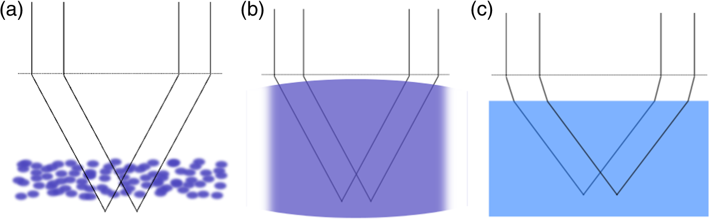 In many biological samples, a substantial cause of aberrations is the refractive index mismatch between the sample immersion medium (PBS, for example) and the organism body.30 This situation is intermediate between Figs. 1(a) and 1(c), but provides a field of view of tens of microns after correction as we show below. Many samples will have a largely cylindrical (C. elegans) or spherical (mouse embryo) shape with a refractive index difference of a few percent. The aberrations across the field of view due to a cylinder or sphere can be modeled using ray tracing.31 In Fig. 2, we show a simulation of the aberrations caused by imaging through a diameter cylinder at a wavelength of 510 nm with a refractive index difference, , relative to the surrounding medium. Rays are traced over the full 60 deg acceptance angle of the objective and the path length along each ray is calculated [Fig. 2(a)]. In Fig. 2(b), the root mean square (RMS) wavefront error is shown across the cylinder. The wavefront error along the center of the cylinder is smallest and is due mostly to astigmatism from the cylindrical shape which acts as a lens. As the imaging point moves toward the edge of the worm, the aberration increases because some of the rays miss the cylinder entirely and some pass through causing a step-like discontinuity in the wavefront as shown in Fig. 2(b). Fig. 2(a) Schematic illustrating the imaging geometry. Rays are traced from point , under the cylinder to the entrance to the imaging objective where the wavefront is calculated. The cylinder has a radius of and a refractive index difference of 0.02 relative to the surrounding medium. The imaging point, , is in a lateral plane directly under the cylinder, and the maximum angle of captured rays is 60 deg. . (b) Map of the RMS wavefront error before correction (radians). The aberration is the greatest at the edge of the cylinder. To the right are the wavefront and PSF at the center (1a, 1b), midway to the edge (2a, 2b), and at the edge of the cylinder (3a, 3b). (c) Map of RMS wavefront error after correction and corresponding wavefronts and PSFs (4a, 4b to 6a, 6b). The numbers in figures (b) and (c) indicate the positions where the wavefronts (1 to 6) are measured. (d) Strehl ratio before (dashed) and after (solid) correction. Scale bar is .  The Strehl ratio varies from 0.22 at the center of the cylinder to halfway to the edge. If we correct for the wavefront at the center [Figs. 2(c) and 2(d)], then the Strehl ratio will vary from 1.0 to 0.025 halfway to the edge. If we define acceptable imaging as a Strehl ratio greater than 0.2, the field of view in the lateral direction goes from less than before correction to almost after correction. 3.Effect of Aberrations on Structured Illumination MicroscopyAs described in detail previously, in 2-D SIM, nine raw images are acquired in order to reconstruct the final high-resolution image.5 The stripe pattern is oriented in three different directions (0, 120, and 240 deg with respect to an arbitrary axis in the lateral plane), and, at each direction, the pattern phase is shifted by 0, 120, and 240 deg. That is, the raw images can be described by the equation where and run from 1 to 3 indicating the angle and phase of the pattern. is the fluorophore density and is the PSF.The raw images are then linearly transformed to separate out the image components centered on frequencies . This can be performed in either the spatial or Fourier domain The final image is then reconstructed in the Fourier domain where is the Fourier transform of , and is the optical transfer function (OTF). In the ideal case, , and , and the reconstructed image is a faithful representation of the object up to spatial frequencies of . When aberrations are present, the OTF is distorted and with similar expressions for where is the aberrated OTF. Now, the effective transfer function is distorted resulting in artifacts in the imageFigure 3 shows the simulations of 2-D SIM reconstructions with noise and aberrations, as well as simulations of widefield and deconvolution images [Figs. 3(a)–3(d)] for comparison. In the SIM reconstructions, as the number of photons decreases and the relative shot noise increases [Figs. 3(e)–3(j)], the parameter must be increased to keep the SNR acceptable, but the resolution still degrades. The effect of noise can be seen in an increase in the signal at the edge of the OTF where the noise, which has a flat frequency response, is boosted by the low value of the OTF in the denominator of Eq. (4). can be increased further to reduce the noise further but at the expense of resolution. Fig. 3Simulations of two-dimensional structured illumination microscopy (SIM) on a field of point objects. The images are sections of larger fields which are used to generate the Fourier transforms (FT). (a and b) Widefield image and FT. Each point emits an average of 10,000 photons at the maximum intensity of the SIM pattern. In (a), the scale bar is 200 nm. In (b), the scale bar is . (c and d) Deconvolved image and FT with an average of 10,000 photons per point; . (e and f) SIM image and FT with an average of 10,000 photons per point; . (g and h) SIM image and FT with an average of 500 photons per point; . (i and j) SIM image and FT with an average of 100 photons per point; . (k and l) SIM image and FT when the image is aberrated by 1 radian RMS of astigmatism, with 10,000 photons per point; . (m and n) SIM image and FT when the image is aberrated by 1 radian RMS of astigmatism, with 500 photons per point; . (o and p) SIM image and FT when the image is aberrated by 1 radian RMS of astigmatism, with 10,000 photons per point, using the aberrated optical transfer function in the reconstruction; . For these simulations, the NA is 1.2 and the wavelength is 510 nm. 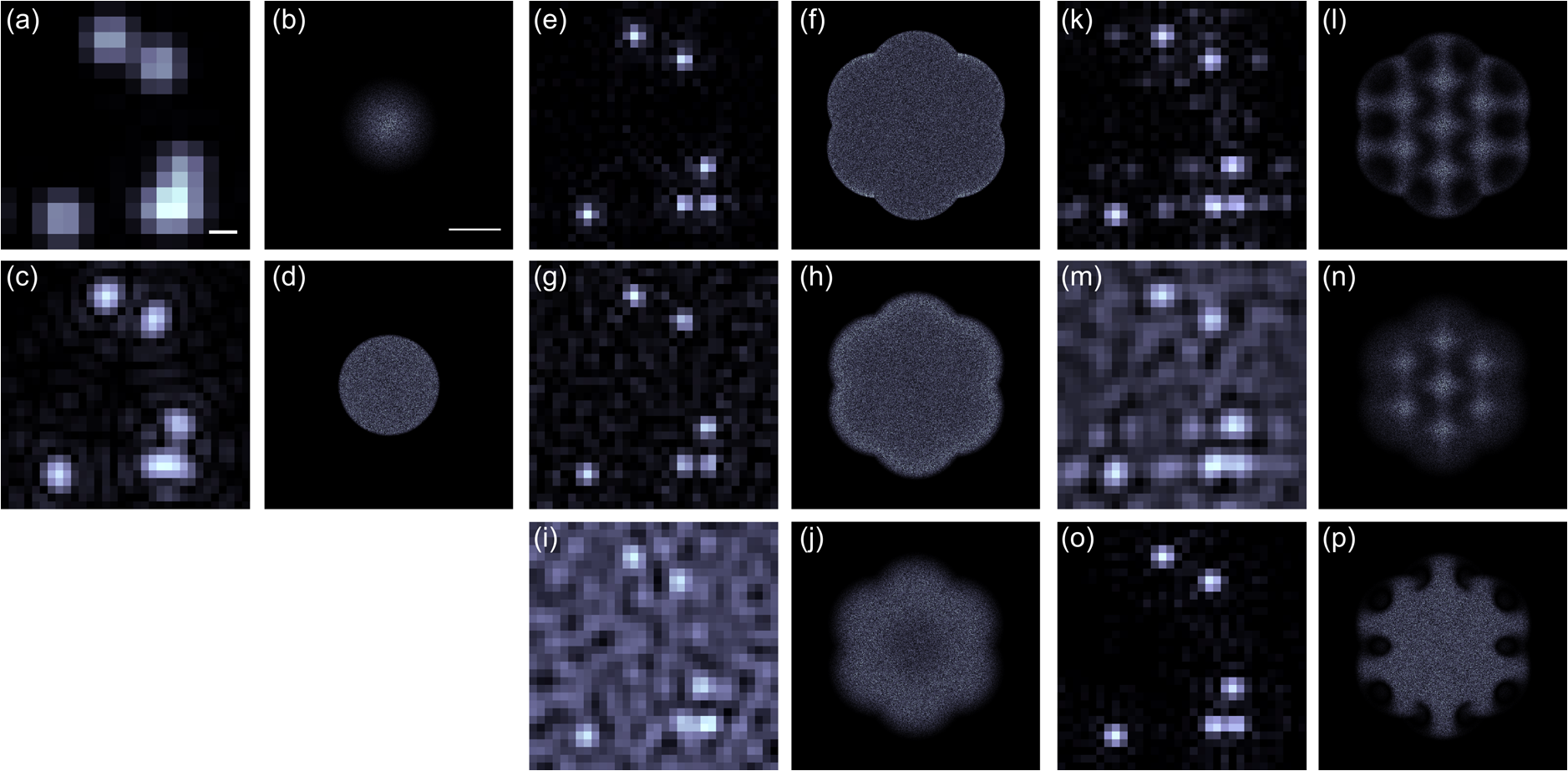 Optical aberrations will reduce the strength of the OTF at high frequencies so there will be gaps in the frequency support which result in artifacts in the image even at high SNR. Here, we show the effect of 1.0 radian RMS of astigmatism [Figs. 3(k)–3(p)]. Even at high SNR [Figs. 3(k) and 3(l)] the aberrations cause significant artifacts in the image. At lower SNR [Figs. 3(m) and 3(n)], the aberrated image is significantly worse than the unaberrated image with comparable SNR [Figs. 3(g) and 3(h)]. The aberrations can be compensated to some extent by using the aberrated OTF in Eq. (4) as shown in Figs. 3(o) and 3(p)]. This requires knowledge of the aberrated OTF and still results in a degraded image. If the aberrated OTF can be determined, it should be corrected, as we discuss below. If the aberrations consist of an isoplanatic component and an anisoplanatic component, the AO system will only correct the isoplanatic aberration, and we can write the corrected system PSF as where cannot be written in the form .32 As an example, the image component will be In the Fourier domain, the anisoplanatic component will result in a term When the image is reconstructed using Eq. (4), the term above will produce a term in the reconstruction These terms will contribute artifacts which will typically look like additional noise in the final image. If , then the artifacts will be small compared to the SIM image, and the reconstruction will be successful. Because the aberrations will reduce the high frequency components in the OTF, these terms will contribute artifacts that are peaked at the spatial frequencies . In the spatial domain, the artifacts will be most pronounced in those areas where is large. This is evident in the data presented in Sec. 4 in comparing the regions under and not under the worm. 4.Experimental Results4.1.Optical SetupA schematic of the AO-SIM system is shown in Fig. 4. We use an Olympus IX71 inverted microscope with a Prior Proscan XY Stage (H117P21X) and a Prior 200 micron travel NanoScan Z stage. The microscope objective is a 1.4NA oil immersion objective (Plan Apo N, Olympus), and the Olympus tube lens has a focal length of 180 mm. The light exits the microscope through the left-side port where the back pupil plane is reimaged onto a deformable mirror (DM) (Mirao 52-e Imagine Optic). The mirror has 52 actuators and is 15 mm in diameter. The objective back pupil plane is reimaged onto the DM with the tube lens and a lens , so that the system NA is limited to 1.285 by the DM. Fig. 4Schematic of the microscope. , , , and . DiM, dichroic mirror; PR, polarization rotator; and DLP, digital light projector.  The image plane is reimaged onto the CCD camera (Ixon, Andor) with an additional magnification factor of 3, so that the pixel size in the sample space is 89 nm, slightly below the Nyquist sampling limit for the system of 100 nm. The sample is excited with a 488 nm laser (Cyan 488, Newport) which is coupled into a core diameter fiber. The fiber is shaken using a fiber shaker as described in Ref. 12 to remove speckle, creating a partially coherent source.8 The structured illumination is created with a Digital Light Projector (DLP) (0.7 in. XGA D4000, Texas Instruments). The polarization is controlled with a linear polarizer (LPVISE100-A, Thorlabs) in a fast motorized stage (8MRU, Altechna) to maintain the polarization normal to the structured illumination direction [ in Eq. (1)] for maximum pattern modulation depth.5 To maintain the optical quality of the structured light, the dichroic mirror is a custom dichroic (Omega Optical) on a 9-mm thick substrate (CVI Laser Optics) to maintain a wavefront that is flat to better than RMS. 4.2.Sample PreparationTo test the AO-SIM system, fluorescent microbeads were dried beneath wildtype C. elegans samples. 200-nm and 100-nm diameter yellow-green fluorescent microbeads (F-8803 and F-8811, Life Technologies, peak emission wavelength of 515 nm) were diluted in ethanol by additional factors of and from their initial concentrations, respectively, and combined. of the solution was dried on the slide. To fix the C. elegans samples, of a solution of the antihelminthic drug tetramisole (L9756, Sigma) was applied to the slide. The worms were then transferred to the slide with inoculating loops. After allowing the tetramisole to dry, of glycerol was deposited on the slide and the coverslip was mounted and fixed. To prevent the microbeads from being washed away from the slide while applying the worms, charged slides (Colorfrost Plus, Shandon) were used. 4.3.Adaptive Optics SystemOur system does not contain a wavefront sensor and we use sensorless AO to optimize the wavefront.33,34 In sensorless AO, the wavefront to be applied to the DM is expanded in a set of orthogonal modes such as the Zernike modes, and mode coefficients are adjusted to optimize an image-based metric such as the image intensity or sharpness.35 Here, we define the DM shape using the Zernike modes,36 and the metric is the peak intensity in a small region of the image containing a 200-nm microbead. We use phase retrieval to measure the DM actuator influence functions and to correct for system aberrations.37 Three-dimensional stacks of a single 200 nm fluorescent microbead are taken in steps from below to above the focus for phase retrieval measurements. To correct for system aberrations, the phase retrieved wavefront is used to set the DM iteratively until the measured wavefront is acceptably flat.38 Typically, the phase retrieval measurement and correction are repeated two or three times. Examples of the wavefront due to a single actuator, the wavefront with the DM actuators at 0, and the wavefront after correction are shown in Fig. 5. After the correction of system aberrations, the Strehl ratio is greater than 0.80 across the entire field of view of the camera for imaging on the coverslip. Fig. 5(a) The influence function from a single actuator measured by phase retrieval. (b) The wavefront phase with the deformable mirror (DM) actuators all set to 0 V. (c) The wavefront phase after correction. This phase corresponds to a Strehl ratio of 0.85.  To obtain deep-tissue, superresolution images, AO correction is first performed by optimizing the intensity of a 200-nm microbead fixed beneath the center of the worm. In the present system, the amplitudes of the low-order Zernike polynomials are sequentially varied coarsely from to 10 radians in 1 radian steps to maximize the bead intensity. To optimize the intensity, a parabolic fit to five data points around the initial estimate is then applied to the intensity data for each Zernike mode, and the mode amplitude corresponding to the maximum is applied to the system.39 The magnitude of the bias aberrations used in the parabolic fit had maximum amplitudes of and radians on each side of the initial estimate. This ensured that the maximum was in range so that the fit performed correctly. Zernike modes 5, 6, 7, 8, and 11, corresponding to astigmatism, coma, and spherical aberration, were corrected sequentially in this manner. 4.4.Structured IlluminationAfter the aberration correction, 2-D SIM was performed following the approach of Gustafsson.5 We use a stripe pattern with a period of 290 nm in image space corresponding to 65% of the numerical aperture. We use a relatively modest stripe period for SIM to provide a greater overlap between and . Although this will reduce the resolution by , we still achieve a resolution of 140 nm. The greater overlap makes it easier to calculate the magnitude and orientation of as well as the initial phase and the modulation depth of the pattern because these values are calculated by comparing the values of and in the region of k-space in which they overlap.5 4.5.ResultsIn Fig. 6, we show images of fluorescent beads below a C. elegans adult hermaphrodite. C. elegans is a model organism used to study a large variety of biological processes including cell signaling, gene regulation, metabolism, drug delivery, and ageing.40–42 A differential interference contrast image of the central longitudinal region of the worm is shown in Fig. 6(a). The width of the worm is approximately . Figures 6(b) and 6(c) show widefield images before and after correction. The final two panels of Figs. 6(d) and 6(e) show the SIM reconstructed images with and without AO correction. As shown in the images, the structured illumination (SI) reconstructions show an increased resolution. However, performing SI reconstruction without AO correction results in a highly distorted image of the microbeads with increased imaging artifacts. Fig. 6(a) Differential interference contrast image showing the intestine of a C. elegans sample. The yellow boxes indicate the regions shown in Figs. 8 and 11. (b) 0.1- and microbeads fixed beneath the sample. (c) Image of the microbeads after adaptive optics (AO) correction. (d) SIM reconstruction after AO correction. (e) SIM reconstruction without AO correction.  Figure 7 shows the aberrations removed from the wavefront by the DM. The dominant aberration is astigmatism as we expect from the shape of the worm. The total RMS wavefront error removed is 2.23 radians. Fig. 7(a) The wavefront removed by the DM. (b) The amplitudes of the Zernike modes applied to the DM. The Zernikes are defined as in Ref. 36.  The differences in resolutions and artifacts are apparent in Fig. 8 which shows a close-up view of three 100-nm microbeads. Without SI [Figs. 8(a) and 8(b)], the microbeads cannot be individually resolved. Without AO correction [Fig. 8(d)], the SIM reconstruction is highly aberrated with increased noise around the beads. In Fig. 8(b), we show the deconvolved widefield image after AO correction to demonstrate that deconvolution does not provide the resolution of SIM although the combination of AO correction and deconvolution is a significant improvement over the uncorrected widefield image [Fig. 8(a)]. Fig. 8Examples of AO-SI. 100-nm microbeads fixed beneath a C. elegans sample—center box in Fig. 6(a). (a) Widefield image before AO correction. (b) Deconvolved widefield image after correction. SI reconstruction with, (c), and without, (d), AO. (e–h) same as (a–d) but another location roughly away. 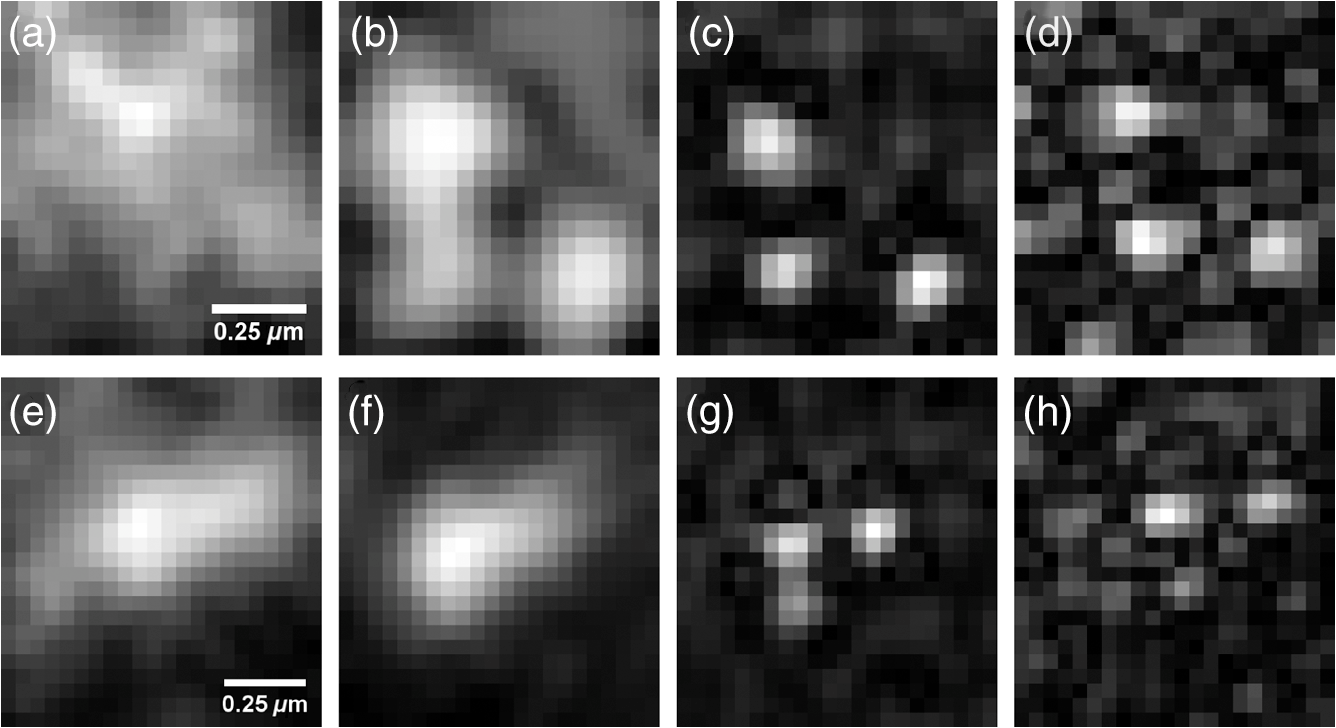 The SNR of the SI reconstructed images in Figs. 8(c) and 8(d) were calculated by taking the top five pixel intensities from the image and the standard deviation of a background area within a few microns. The SNR without AO correction is 13.3. With AO correction, the SNR increases to 21.5. We have verified that the improvement in SNR is only weakly dependent on the parameter from Eq. (4). The plot in Fig. 9 is a profile in the horizontal direction through the beads displayed at the bottom of Figs. 8(a)–8(c). The peak intensity is doubled by removing the aberrations with AO and quadrupled with SIM when compared to the corrected widefield image. With AO and SI, the measured full width at half maximum of a 100-nm microbead is 140 nm. Fig. 9Profiles of two 100-nm microbeads fixed beneath the C. elegans sample. These are the two beads in the lower half of Figs. 8(a)–8(c). WF, widefield without AO; WFAO, widefield with AO; and SIAO, SI image with AO.  A concern with using AO with widefield microscopy techniques is that the correction will only apply to a small field of view. In Fig. 10, we plot the average bead intensity in a transverse (dorsal-ventral) direction across the worm body. (In a tetramisole solution, the paralyzed worms lie with their left or right lateral sides touching the slide.) This was accomplished by taking image slices that were 48 pixels in the vertical direction and 256 pixels in the horizontal direction through the center of the image and recording the average of the top 5 pixel intensities for each slice. The average intensity increase is 60% across the dorsal-ventral width of the worm. (This average includes the top and bottom horizontal slices in which many microbeads are not imaged through the worm.) Along the worm anterior-posterior axis, the improvement extends over , nearly the entire range captured by the imaging camera. In Fig. 11, we show images of 100 nm beads near the edge of the worm (about from the worm’s axis) before and after correction with AO as well as the corresponding SI reconstructions. Here, the importance of the combination of AO and SI is even more evident. The SI image without AO does not correctly identify the 100 nm beads in the field. Fig. 10Average bead intensity across the C. elegans sample in the vertical direction before (blue, open circles) and after (green, closed circles) correction. Each point is calculated by taking the average of the top five pixel intensities from a horizontal strip 48 pixels () wide. 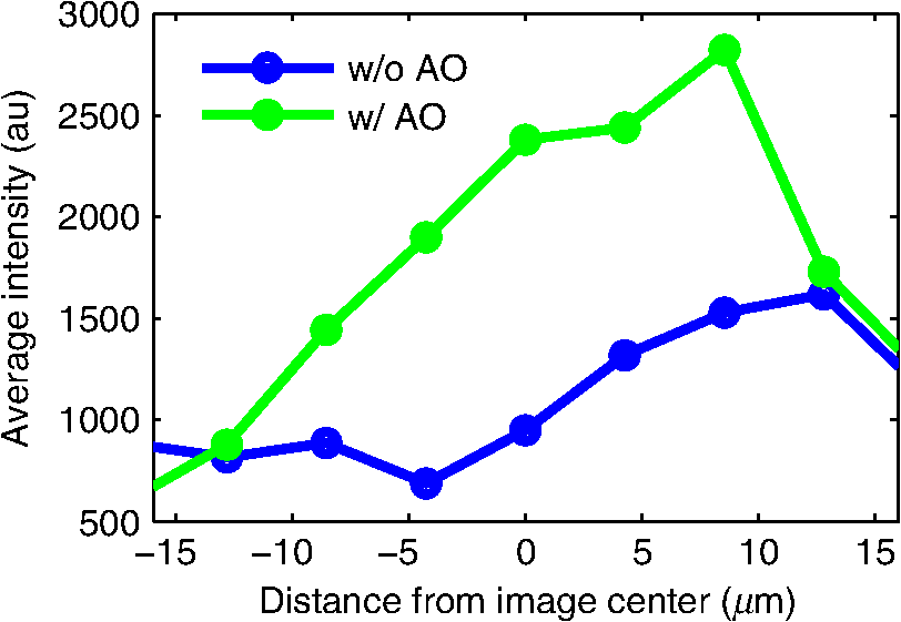 Fig. 11100-nm microbeads near edge of C. elegans body—top box in Fig. 6(a). (a) Widefield image before AO correction. (b) After correction. (c) SI image with AO. (d) SI image without AO.  5.ConclusionIn conclusion, we have demonstrated a microscope system that provides resolution beyond the diffraction limit through thick tissue by combining AO-SIM. A resolution of 140 nm through of tissue can be achieved. AO-SI increases the peak intensity of point objects by a factor of 4. Depending on the magnitude of the aberrations, SIM may not be possible without AO. Even if SIM reconstruction works when imaging through thick tissue, the correction of aberrations with AO can substantially improve the SNR. Although AO has previously been combined with SIM, that work focused on the development of sensorless AO for use with optically sectioned SIM images, and did not present the enhanced resolution.28 140-nm resolution has also been demonstrated in thick samples without AO using a version of SIM based on image scanning microscopy,22,43 but without AO. Here, we combine AO and SIM to achieve high resolution in highly aberrating conditions. Whereas, with scanning microscopy techniques, the aberrations can be corrected, at least in principle, on a point by point basis, in widefield and SIM, the entire field of view is captured at once using one wavefront correction. We show that AO greatly improves the image quality of the SI image over a field of view. This improvement is due to a single correction based on one bead near the center of the image. In the event that the corrected field of view is not large enough, different corrections can be applied for different areas of the image, and the images could be combined by image fusion.44 Multiconjugate AO can also be used to increase the corrected field of view.45 Future work will involve applying 3-D AO-SIM to fluorescently labeled C. elegans. AcknowledgmentsThis research was supported by the University of Georgia Research Foundation, a Ralph E. Powe Junior Faculty Enhancement Award, and the National Science Foundation under Grant MCB1052672. ReferencesS. W. Hell and J. Wichmann,
“Breaking the diffraction resolution limit by stimulated emission: stimulated-emission-depletion fluorescence microscopy,”
Opt. Lett., 19
(11), 780
–782
(1994). http://dx.doi.org/10.1364/OL.19.000780 OPLEDP 0146-9592 Google Scholar
E. Betzig et al.,
“Imaging intracellular fluorescent proteins at nanometer resolution,”
Science, 313
(5793), 1642
–1645
(2006). http://dx.doi.org/10.1126/science.1127344 SCIEAS 0036-8075 Google Scholar
S. T. Hess, T. P. K. Girirajan and M. D. Mason,
“Ultra-high resolution imaging by fluorescence photoactivation localization microscopy,”
Biophys. J., 91
(11), 4258
–4272
(2006). http://dx.doi.org/10.1529/biophysj.106.091116 BIOJAU 0006-3495 Google Scholar
M. J. Rust, M. Bates and X. Zhuang,
“Sub-diffraction-limit imaging by stochastic optical reconstruction microscopy (STORM),”
Nat. Methods, 3
(10), 793
–796
(2006). http://dx.doi.org/10.1038/nmeth929 1548-7091 Google Scholar
M. G. Gustafsson,
“Surpassing the lateral resolution limit by a factor of two using structured illumination microscopy,”
J. Microsc., 198
(2), 82
–87
(2000). http://dx.doi.org/10.1046/j.1365-2818.2000.00710.x JMICAR 0022-2720 Google Scholar
G. Donnert et al.,
“Macromolecular-scale resolution in biological fluorescence microscopy,”
Proc. Natl. Acad. Sci. U. S. A., 103
(31), 11440
–11445
(2006). http://dx.doi.org/10.1073/pnas.0604965103 PNASA6 0027-8424 Google Scholar
R. Heintzmann and C. G. Cremer,
“Laterally modulated excitation microscopy: improvement of resolution by using a diffraction grating,”
Proc. SPIE, 3568 185
–196
(1999). http://dx.doi.org/10.1117/12.336833 PSISDG 0277-786X Google Scholar
M. G. L. Gustafsson et al.,
“Three-dimensional resolution doubling in wide-field fluorescence microscopy by structured illumination,”
Biophys. J., 94
(12), 4957
–4970
(2008). http://dx.doi.org/10.1529/biophysj.107.120345 BIOJAU 0006-3495 Google Scholar
M. G. Gustafsson,
“Nonlinear structured-illumination microscopy: wide-field fluorescence imaging with theoretically unlimited resolution,”
Proc. Natl. Acad. Sci. U. S. A., 102
(37), 13081
–13086
(2005). http://dx.doi.org/10.1073/pnas.0406877102 PNASA6 0027-8424 Google Scholar
E. H. Rego et al.,
“Nonlinear structured-illumination microscopy with a photoswitchable protein reveals cellular structures at 50-nm resolution,”
Proc. Natl. Acad. Sci. U. S. A., 109
(3), E135
–E143
(2012). http://dx.doi.org/10.1073/pnas.1107547108 PNASA6 0027-8424 Google Scholar
P. Kner et al.,
“Super-resolution video microscopy of live cells by structured illumination,”
Nat. Methods, 6
(5), 339
–342
(2009). http://dx.doi.org/10.1038/nmeth.1324 1548-7091 Google Scholar
L. Shao et al.,
“Super-resolution 3D microscopy of live whole cells using structured illumination,”
Nat. Methods, 8
(12), 1044
–1046
(2011). http://dx.doi.org/10.1038/nmeth.1734 1548-7091 Google Scholar
M. J. Booth,
“Adaptive optics in microscopy,”
Philos. Trans. A, 365
(1861), 2829
–2843
(2007). http://dx.doi.org/10.1098/rsta.2007.0013 PTRMAD 1364-503X Google Scholar
T. J. Gould et al.,
“Adaptive optics enables 3D STED microscopy in aberrating specimens,”
Opt. Express, 20
(19), 20998
–21009
(2012). http://dx.doi.org/10.1364/OE.20.020998 OPEXFF 1094-4087 Google Scholar
M. J. Booth et al.,
“Adaptive aberration correction in a confocal microscope,”
Proc. Natl. Acad. Sci. U. S. A., 99
(9), 5788
–5792
(2002). http://dx.doi.org/10.1073/pnas.082544799 PNASA6 0027-8424 Google Scholar
X. Tao et al.,
“Live imaging using adaptive optics with fluorescent protein guide-stars,”
Opt. Express, 20
(14), 15969
–15982
(2012). http://dx.doi.org/10.1364/OE.20.015969 OPEXFF 1094-4087 Google Scholar
L. Sherman et al.,
“Adaptive correction of depth-induced aberrations in multiphoton scanning microscopy using a deformable mirror,”
J. Microsc., 206
(1), 65
–71
(2002). http://dx.doi.org/10.1046/j.1365-2818.2002.01004.x JMICAR 0022-2720 Google Scholar
D. Débarre et al.,
“Image-based adaptive optics for two-photon microscopy,”
Opt. Lett., 34
(16), 2495
–2497
(2009). http://dx.doi.org/10.1364/OL.34.002495 OPLEDP 0146-9592 Google Scholar
P. Kner et al.,
“High-resolution wide-field microscopy with adaptive optics for spherical aberration correction and motionless focusing,”
J. Microsc., 237
(2), 136
–147
(2010). http://dx.doi.org/10.1111/jmi.2010.237.issue-2 JMICAR 0022-2720 Google Scholar
O. Azucena et al.,
“Adaptive optics wide-field microscopy using direct wavefront sensing,”
Opt. Lett., 36
(6), 825
–827
(2011). http://dx.doi.org/10.1364/OL.36.000825 OPLEDP 0146-9592 Google Scholar
L. Gao et al.,
“Noninvasive imaging beyond the diffraction limit of 3D dynamics in thickly fluorescent specimens,”
Cell, 151
(6), 1370
–1385
(2012). http://dx.doi.org/10.1016/j.cell.2012.10.008 CELLB5 0092-8674 Google Scholar
A. G. York et al.,
“Resolution doubling in live, multicellular organisms via multifocal structured illumination microscopy,”
Nat. Methods, 9
(7), 749
–754
(2012). http://dx.doi.org/10.1038/nmeth.2025 1548-7091 Google Scholar
F. Cella Zanacchi et al.,
“Live-cell 3D super-resolution imaging in thick biological samples,”
Nat. Methods, 8
(12), 1047
–1049
(2011). http://dx.doi.org/10.1038/nmeth.1744 1548-7091 Google Scholar
N. T. Urban et al.,
“STED nanoscopy of actin dynamics in synapses deep inside living brain slices,”
Biophys. J., 101
(5), 1277
–1284
(2011). http://dx.doi.org/10.1016/j.bpj.2011.07.027 BIOJAU 0006-3495 Google Scholar
K. F. Tehrani and P. Kner,
“Point spread function optimization for STORM using adaptive optics,”
Proc. SPIE, 8978 89780I
(2014). http://dx.doi.org/10.1117/12.2040390 PSISDG 0277-786X Google Scholar
B. R. Patton, D. Burke and M. J. Booth,
“Adaptive optics from microscopy to nanoscopy,”
Proc. SPIE, 8948 894802
(2014). http://dx.doi.org/10.1117/12.2041210 PSISDG 0277-786X Google Scholar
M. A. A. Neil, R. Juskaitis and T. Wilson,
“Method of obtaining optical sectioning by using structured light in a conventional microscope,”
Opt. Lett., 22
(24), 1905
–1907
(1997). http://dx.doi.org/10.1364/OL.22.001905 OPLEDP 0146-9592 Google Scholar
D. Débarre et al.,
“Adaptive optics for structured illumination microscopy,”
Opt. Express, 16
(13), 9290
–9305
(2008). http://dx.doi.org/10.1364/OE.16.009290 OPEXFF 1094-4087 Google Scholar
M. J. Booth, M. A. A. Neil and T. Wilson,
“Aberration correction for confocal imaging in refractive-index-mismatched media,”
J. Microsc., 192
(2), 90
–98
(1998). http://dx.doi.org/10.1111/j.1365-2818.1998.99999.x JMICAR 0022-2720 Google Scholar
M. Schwertner, M. Booth and T. Wilson,
“Characterizing specimen induced aberrations for high NA adaptive optical microscopy,”
Opt. Express, 12
(26), 6540
–6552
(2004). http://dx.doi.org/10.1364/OPEX.12.006540 OPEXFF 1094-4087 Google Scholar
M. Schwertner, M. J. Booth and T. Wilson,
“Simulation of specimen-induced aberrations for objects with spherical and cylindrical symmetry,”
J. Microsc., 215
(3), 271
–280
(2004). http://dx.doi.org/10.1111/j.0022-2720.2004.01371.x JMICAR 0022-2720 Google Scholar
J. W. Goodman, Statistical Optics, 1st ed.Wiley Interscience, New York
(1985). Google Scholar
M. J. Booth,
“Wave front sensor-less adaptive optics: a model-based approach using sphere packings,”
Opt. Express, 14
(4), 1339
–1352
(2006). http://dx.doi.org/10.1364/OE.14.001339 OPEXFF 1094-4087 Google Scholar
M. J. Booth,
“Wavefront sensorless adaptive optics for large aberrations,”
Opt. Lett., 32
(1), 5
–7
(2007). http://dx.doi.org/10.1364/OL.32.000005 OPLEDP 0146-9592 Google Scholar
S. P. Poland, A. J. Wright and J. M. Girkin,
“Evaluation of fitness parameters used in an iterative approach to aberration correction in optical sectioning microscopy,”
Appl. Opt., 47
(6), 731
–736
(2008). http://dx.doi.org/10.1364/AO.47.000731 APOPAI 0003-6935 Google Scholar
R. J. Noll,
“Zernike polynomials and atmospheric turbulence,”
J. Opt. Soc. Am., 66
(3), 207
–211
(1976). http://dx.doi.org/10.1364/JOSA.66.000207 JOSAAH 0030-3941 Google Scholar
B. M. Hanser et al.,
“Phase retrieval for high-numerical-aperture optical systems,”
Opt. Lett., 28
(10), 801
–803
(2003). http://dx.doi.org/10.1364/OL.28.000801 OPLEDP 0146-9592 Google Scholar
P. Kner et al.,
“Closed loop adaptive optics for microscopy without a wavefront sensor,”
Proc. SPIE, 7570 757006
(2010). http://dx.doi.org/10.1117/12.840943 PSISDG 0277-786X Google Scholar
M. J. Booth, D. Débarre and T. Wilson,
“Image-based wavefront sensorless adaptive optics,”
Proc. SPIE, 6711 671102
(2007). http://dx.doi.org/10.1117/12.733635 PSISDG 0277-786X Google Scholar
A. Fire et al.,
“Potent and specific genetic interference by double-stranded RNA in Caenorhabditis elegans,”
Nature, 391
(6669), 806
–811
(1998). http://dx.doi.org/10.1038/35888 NATUAS 0028-0836 Google Scholar
S. S. Lee et al.,
“DAF-16 target genes that control C. elegans life-span and metabolism,”
Science, 300
(5619), 644
–647
(2003). http://dx.doi.org/10.1126/science.1083614 SCIEAS 0036-8075 Google Scholar
T. Kaletta and M. O. Hengartner,
“Finding function in novel targets: C. elegans as a model organism,”
Nat. Rev. Drug. Discov., 5
(5), 387
–398
(2006). http://dx.doi.org/10.1038/nrd2031 NRDDAG 1474-1776 Google Scholar
C. B. Müller and J. Enderlein,
“Image scanning microscopy,”
Phys. Rev. Lett., 104
(19), 198101
(2010). http://dx.doi.org/10.1103/PhysRevLett.104.198101 PRLTAO 0031-9007 Google Scholar
J. Swoger et al.,
“Multi-view image fusion improves resolution in three-dimensional microscopy,”
Opt. Express, 15
(13), 8029
–8042
(2007). http://dx.doi.org/10.1364/OE.15.008029 OPEXFF 1094-4087 Google Scholar
Z. Kam et al.,
“Modelling the application of adaptive optics to wide-field microscope live imaging,”
J. Microsc., 226
(1), 33
–42
(2007). http://dx.doi.org/10.1111/jmi.2007.226.issue-1 JMICAR 0022-2720 Google Scholar
BiographyBenjamin Thomas completed his PhD degree in engineering at the University of Georgia in December 2014. He received his BS and MS degrees in engineering from the University of Georgia in 2008 and 2011, respectively. |


