1.

Introduction

Optical coherence tomography (OCT) is a noninvasive high-resolution imaging technology that has been widely applied in probing the microstructure of biological tissue.^1–3 Human retinal imaging is the most successful clinical application of OCT. OCT has greatly improved the early diagnosis of retinal diseases and is highly valuable in the diagnosis of macular holes, cystoid macular edema, diabetic retinopathy, and age-related macular degeneration. OCT is based on the principle of low-coherence interferometry, the imaging results are sensitive to speckle noise (i.e., signal-degrading speckle),^4,5 which reduces the quality and blurs the feature details of obtained images.^6,7

Many speckle noise reduction techniques involving hardware-based and software-based methods have been proposed. Hardware-based methods aim to acquire multiple tomograms with uncorrelated speckle patterns. Uncorrelated speckle patterns can be obtained with different angles, positions, and frequencies or by compressing the sample such as by angular compounding,⁸ spatial compounding,⁹ frequency compounding,¹⁰ and strain compounding.¹¹ However, these hardware-based methods require additional optical components or modification of the sample arm, and these methods cannot be easily applied to a commercial OCT system. Software-based methods are postprocessing techniques used after an image is acquired. These methods use some form of smoothing filter in an image or by multiple uncorrelated images averaging to reduce speckle. One problem of these software-based methods is that it may reduce resolution of the image. Given that the software-based methods do not change the optical configuration and can be directly applied to an OCT system, many image postprocessing methods, such as median and wiener filters,¹² wavelet transformations,^13,14 curvelet shrinkage,^15,16 iterative sparse reconstruction,¹⁷ and multiple uncorrelated B-scans averaging,¹⁸ have been proposed.

Under the B-scan averaging method, the signal-to-noise ratio (SNR) of the resulting image is increased as the square root of the number of averaged B-scans if the speckle is uncorrelated between images.⁴ When OCT retinal imaging is being performed, the human eye will move unconsciously such as nystagmus and microsaccades. Even during conscious visual fixation, the “fixational eye movements” are unavoidable.¹⁹ Such movements lead to the change of speckle patterns of a series of successive recorded images and decorrelation of the speckle noise of the recorded retinal B-scans. The speckle noise can be reduced by averaging these images. The main challenge of the multiple uncorrelated B-scans averaging method is the alignment of recorded multiple B-scans to compensate for sample motion. Any misalignment reduces the spatial resolution of the average image and affects the identification of clinical features. Image registration accuracy can be improved by combination with a real-time eye tracking system.²⁰ However, this additional system can only compensate for lateral displacements and increases scanning times. Jorgensen and Thomadsen¹⁸ proposed an OCT image registration method based on the regularized shortest path algorithm with an axial-to-lateral registration iterative scheme. However, this method cannot align images with large lateral displacements²¹ and cannot correct for rotation. Alonso-Caneiro et al.²² introduced a registration method by affine-motion model, which can account for higher degrees of image transformations. However, it requires a high level of computational complexity and thus may be unsuitable for real-time operation. Antony et al.²³ presented a registration method where the surface between the inner and outer segments of the photoreceptor cells is used with two stage thin-plate splines to correct for axial artifacts. Chen et al.²⁴ introduced a method that uses the top and bottom boundaries of the retina to aid in registration with a deformable axial registration using a one-dimensional (1-D) radial basis functions. These two registration methods required a segmentation of the B-scan image to guide the registration method. This requirement restricts the registration accuracy because of the accuracy of segmentation algorithm.

In this paper, we propose a two-step method for OCT image registration that combines global and local registrations. In the first step, we register the images based on the rigid transformation model. In the second step, a graph-based algorithm is used to find the optimal shifts along the axial direction of the individual A-scans in the image to align both scans. The results of this method in the imaging of the human retina are discussed in this paper.

2.

Principles

For two given images, where one is a reference image $I(x,y)$ and the other is a warped image $J(u,v)$, the main registration task is to determine an optimal spatial transformation model $T$ such that the images $I$ and $\tilde{J}$ are as similar as possible. $\tilde{J}$ is defined as

2.2.

Local Registration

Local displacements are corrected by determining axial shifts at each corresponding A-scan in B-scan images. In local registration, we are concerned about axial local shifts because the retinal images have an inherent horizontal structure, and the lateral local shifts are not obvious after global registration. A graph-based algorithm is applied to find the optimal relative shifts of the individual A-scans between the reference and warped images. The cost image used to construct the graph is based on the cross-correlation between aligning A-scans in both images at different shifts. Given the presence of speckle noise and other noises, the relative shifts obtained by searching for the maximum cross-correlation are not always the optimum registration values. Considering the spatial continuity of the retinal structure, axial shifts of the adjacent A-scan must be very continuous and smooth. So, we take the relative shifts of adjacent A-scans into account while finding the optimal relative shifts of each A-scan.

The graph $X(n,j)$ is formed by calculating the negative cross-correlation for possible shifts of each corresponding column in the reference image $I$ and warped image $J$. The size of images $I$ and $J$ is $M\times N$, where $M$ are the rows and $N$ are the columns of each image. The image $X$ of the $j$’th column is defined as

Eq. (6)

$$X(n,j)=-\sum _{i=1}^{M-n}\frac{1}{M-n}I(i+n,j)·J(i,j),n\ge 0,$$

Eq. (7)

$$X(n,j)=-\sum _{i=1}^{M-n}\frac{1}{M-n}I(i,j)·J(i-n,j),n<0,$$

where $n$ is the relative shift of the $j$’th column and the value range of $n$ is ($-M$, $M$). The graph search method finds the cost path in the cost image for which the total negative cross-correlation value is minimal.

Eq. (8)

$$Y=\sum _{j=1}^{N}X(n,j).$$

We do not allow large jumps in the found path, so a penalty term for roughness is added to the cost path to constrain roughness. The roughness of the cost path is defined as

Eq. (9)

$$Y_{\text{smooth}}=\sum _{j=2}^{N-1}{(n_{j-1}+n_{j+1}-2n_j)}^2.$$

A new definition of the cost path is

Eq. (10)

$$Y_{\mathrm{new}}=Y+\lambda Y_{\text{smooth}}=\sum _{j=1}^{N}X(n,j)+\lambda \sum _{j=2}^{N-1}{(n_{j-1}+n_{j+1}-2n_j)}^2,$$

where $\lambda$ is a regularization constant. When $Y_{\text{new}}$ is minimal, the axial shifts $n_j$ of each column are obtained. The penalty term shown in Eq. (9) is minimized, and the cost path is considered smooth according to the definition; however, the path is not really “smooth.” Smoothness is influenced by the discrete spatial nature of the digital image.

To improve the smoothness of the path, a method based on pixel subdivision is proposed. Figure 1 shows the effect of pixel subdivision. Figure 1(a) shows a simplified path composed of a series of gray boxes. The rows of gray boxes in each column indicate the axial shifts $n_j$. According to Eq. (9), the roughness of the path in Fig. 1(a) is $3\lambda$. Pixels in the vertical direction subdivided by the subdivision factor $m=2$ are shown in Fig. 1(b). The new path obtained after pixel subdivision is shown in Fig. 1(c), and the roughness of the new path is zero.

Fig. 1

(a) Simplified path; (b) with pixel subdivision; and (c) new path after pixel subdivision.

The basic idea of pixel subdivision is the axial division of each pixel (vertically) into $m$ subpixels, where $m$ is the subdivision factor, followed by the determination of all columns with different axial shifts compared with the closest column to the left ($|n_j-n_{j-1}|\ne 0$). Finally, shifts are allocated to $m-1$ pixels at the left of the column. The new axial shifts $n_j^{\prime }$ of each column are

Eq. (11)

$$n_{j-y}^{\prime }=n_{j-y}+\frac{y}{m}(n_j-n_{j-1}),y=\mathrm{0,1}\dots m.$$

Because the new axial shifts of each column are not always integers, we must calculate the new gray value of each pixel using the interpolation method.

3.

Experiments and Results

The algorithm was tested on an independent dataset of retinal OCT images centered on the macula taken from 8 healthy subjects and 13 patients, in which each subject had 70 successive B-scans. The OPKO Spectral OCT/SLO instrument was used to record the OCT data. The center wavelength of the light source is 830 nm with a bandwidth of 20 nm. The proposed image registration method was used to align 70 successive B-scans. Figure 2 shows an example of three consecutive B-scan images of the human retina. Displacements in retinal structure among the images are highly apparent. Large displacements are more likely to occur if the patient has problems in fixating on a spot. The average of two B-scan images after global registration is shown in Fig. 4(a). The arrow shows the local displacements of two B-scans. Large displacements between B-scan images are corrected via global registration.

Fig. 2

Multiple consecutive B-scan images of the human retina.

Figure 3(a) shows a B-scan image obtained through the graph-based algorithm during local registration. The smoothness of the path is influenced by the discrete spatial nature of the digital image. This is embodied by “break” phenomena occurring at the two adjacent columns, where the relative axial shifts differ $|n_j-n_{j-1}|\ne 0$. “Break” phenomena are shown by arrows in Fig. 3(a). These phenomena cause discontinuities in the layered retinal structure and influence estimations of the retinal thickness of each layer in the average image. The layered retinal structure becomes smoother after pixel subdivision, as shown in Fig. 3(b). Figure 4(b) shows the average image of the two B-scans after local registration. Figures 4(c) and 4(d), respectively, show the magnified images of the rectangular boxes in Figs. 4(a) and 4(b). The layered retinal structure is blurred in Figs. 4(c) and 4(d). Local displacements are compensated and the images are aligned after local registration.

Fig. 3

(a) Optical coherence tomography (OCT) image obtained through the regularized shortest path algorithm during local registration; the arrows denote “break” phenomena. (b) Image obtained through pixel subdivision (subdivision factor).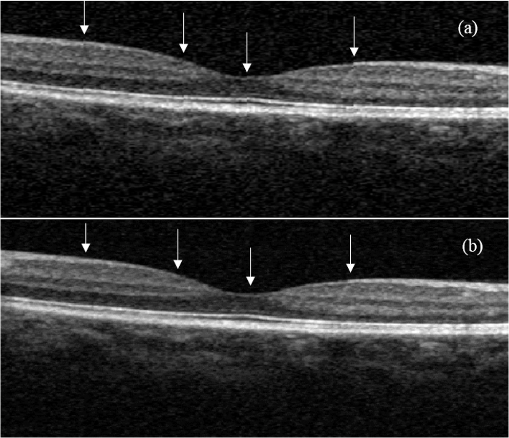

Fig. 4

(a) Average of two images obtained after global registration; the arrow denotes the local displacement of the two images. (b) Average of two images obtained after global and local registrations. (c) and (d) show the magnified images of the rectangular boxes in (a) and (b), respectively.

The computational cost of the local registration algorithm is $O[{(2p+1)}^2·M·N]$, where ($-M,M$) is the value range of $n_j$. Given that nearly all the local displacements are less than 10 pixels, we can limit the value range of $n_j$ to improve the algorithm efficiency. Here, we chose $-10<n_j<10$ to reduce computational costs ($M$ is usually much larger than 10).

A single B-scan from a healthy subject is shown in Fig. 5(a), and the final aligned average of 30 B-scans is shown in Fig. 5(b). The structure of the retinal layers is shown more clearly in the averaged image. To assess the performance of the proposed method, we used signal-to-noise ratio (SNR) and contrast-to-noise ratio (CNR) to measure the image quality quantitatively. The SNR is defined as⁸

Fig. 5

OCT B-scan images of the human retina from a healthy subject: (a) single B-scan and (b) average image obtained after global and local image registrations. NFL: nerve fiber layer; GCL: ganglion cell layer; IPL: inner plexiform layer; INL: inner nuclear layer; OPL: outer plexiform layer; ONL: outer nuclear layer; ELM: external limiting membrane; IS/OS: inner and outer segment junctions of the photoreceptor; and RPE: retinal pigmented epithelium.

Figure 6 shows the improvements in SNR and CNR as functions of the number of averaged images. The method proposed in this study performs better than that proposed in Ref. 18 in terms of both SNR and CNR. SNR improvement in our method closely resembles the square root of $N$, which is the number of averaged images. A factor of around 11 can be obtained during CNR improvement when the number of averaged B-scan images is around 15. The CNR does not show obvious improvement when over 15 images are used, as shown in the figure.

Fig. 6

Improvements in signal-to-noise ratio (SNR) and contrast-to-noise ratio (CNR) as functions of the number of averaged images.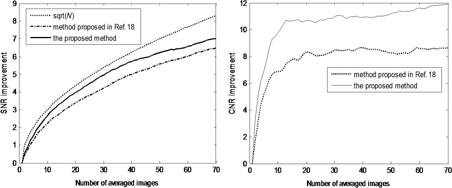

To assess the performance of the loss of spatial resolution brought by our technique, we compared the profile of the inner and outer segment junctions (IS/OS) layer taken from a single A-scan of a single image and an averaged image. Figure 7 presents a region of the IS/OS layer taken from a single A-scan at the foveal region as the white line shown in Fig. 5(a). We measured the full-width-at-half-maximum of the profile, and the profile broadens by about $2\mu \mathrm{m}$ in the averaged 30 B-scan images. It shows that the loss of spatial resolution in the proposed technique is very small compared with the resolution of the system (i.e., $15\mu \mathrm{m}$). Although there is some slight loss of spatial resolution in the averaged image, the reduction of noise makes the structure of the retinal layers clearer [Fig. 5(b)].

Fig. 7

The IS/OS layer taken from a single A-scan at the foveal region [as the white line shown in Fig. 5(a)] of single image and averaged image.

4.

Conclusions

A method for speckle reduction in OCT by combining global and local image registrations has been proposed in this paper. The method does not rely on any information about the retinal layer boundaries and is able to correct translation, rotation, and local deformation in the axial direction. The experimental results showed that the proposed method is an efficient way to align successive images and provides speckle reduction. An SNR improvement of nearly $\sqrt{N}$ and a CNR improvement of around 11 were obtained. The application of this method to align and average OCT images leads to improvements in image quality, which could be beneficial for the identification of retinal structures and clinical diagnosis.